Daniel Mitterdorfer

I currently work on the backend of Elastic Univeral Profiling, which is a fleet-wide continuous profiler. At Elastic we live the concept of space-time, which means that we regularly get to experiment in a little bit similar vein to Google’s 20% time. Mostly recently, I’ve experimented with possibilities to either store less profiling data or query data in a way that allows us to reduce latency. The data model consists basically of two entities:

• Every time our agent captures a stack trace sample, we store this as a profiling event. Each profiling event contains a timestamp, metadata and a reference to a stacktrace index.
• Stacktraces (and a few related data) are stored in separate indices, which we need to retrieve via key-value lookups.

Experiment

When we create a flamegraph in the UI, we filter for a sample of the relevant events and then amend them with the corresponding stacktraces via key-value lookups. These key-value lookups take a significant amount of the overall time so I’ve randomly downsampled stacktraces, put them in separate indices and benchmarked whether the smaller index size led to a reduction in latency. Unfortunately, I could not observe any improvements.

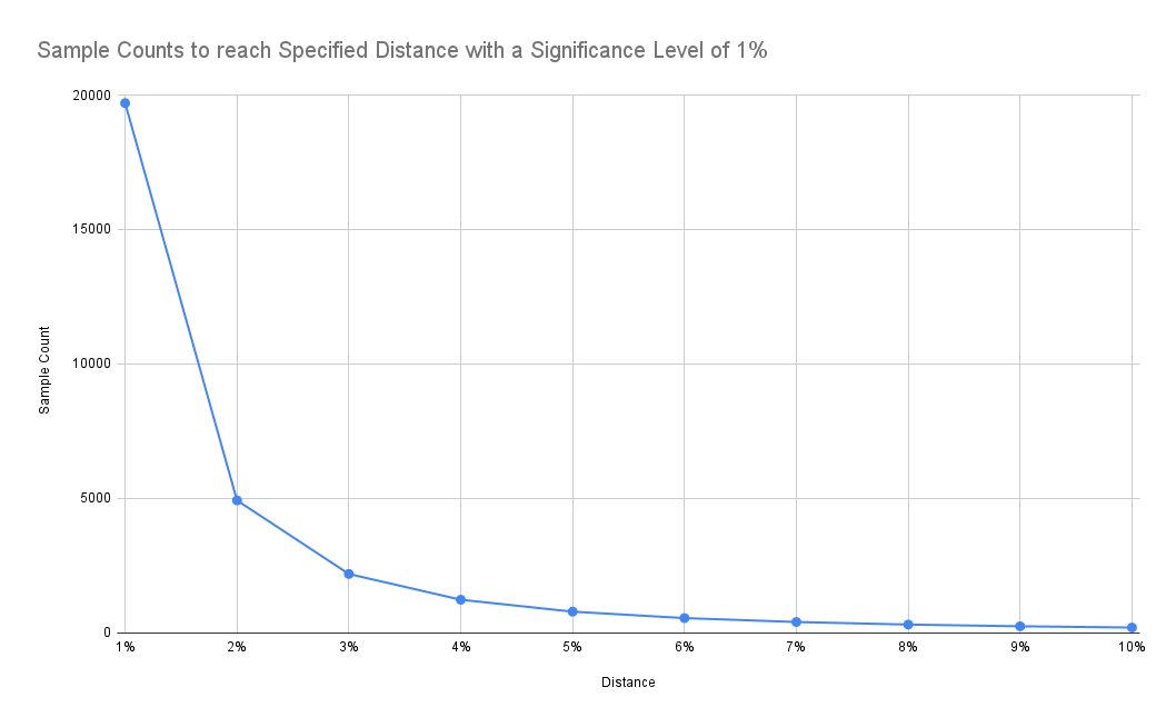
Therefore, I’ve pivoted to better understand the sample size we have chosen to retrieve raw data for flamegraphs (it’s 20.000 samples). The formula to determine the sample size is derived from the paper Sample Size for Estimating Multinomial Proportions. The paper describes an approach to determine the sample count for a multinomial distribution (i.e. stackstraces) with a specified significance level α and a maximum distance d from the true underlying distribution. We have chosen α=0.01 and d=0.01. The formula to calculate sample size n is calculated as:

n=1.96986/d²

The value 1.96986 for the significance level α=0.01 is taken directly from the paper. If you don’t have access, see also this post for more background.

If we are accepting a higher distance from the underlying distribution, we can see that required sample size reduces significantly:

Results

As expected, latency drops as we increase the tolerated distance. Note that the y-axis in the chart below is log-scale:

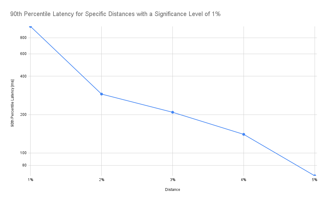
According to the chart above, accepting a 2% distance (instead of 1%) results in a drop of the 90th percentile latency from 982ms to 289ms, i.e. it takes 70% less time to retrieve the data. In addition, the frontend also needs to process only a fraction of the data.

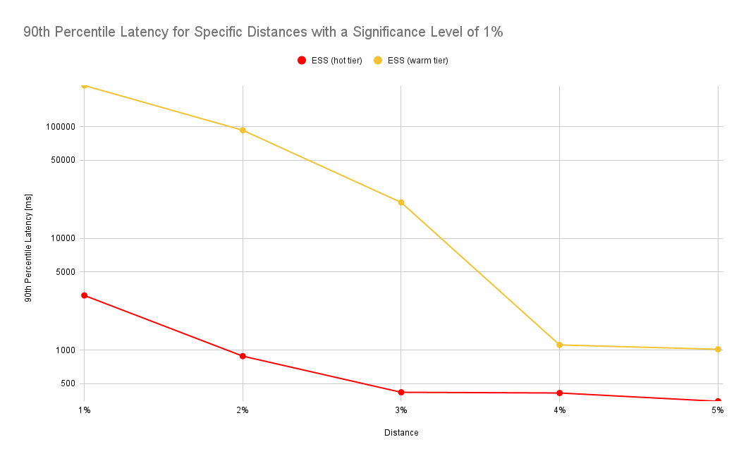
The numbers look similar for a different experiment where we force all indices to be on the hot or warm tier of a cluster. In this benchmark we’ve used a different scenario where we’ve queried a much larger data set covering an entire month whereas in the prior experiment we’ve only queried a day worth of data:

Evaluation

The results look promising but this begs the question whether a 2% distance is acceptable in practice. Therefore, we’ve compared flamegraphs with different distances visually. So let’s look first at our baseline.

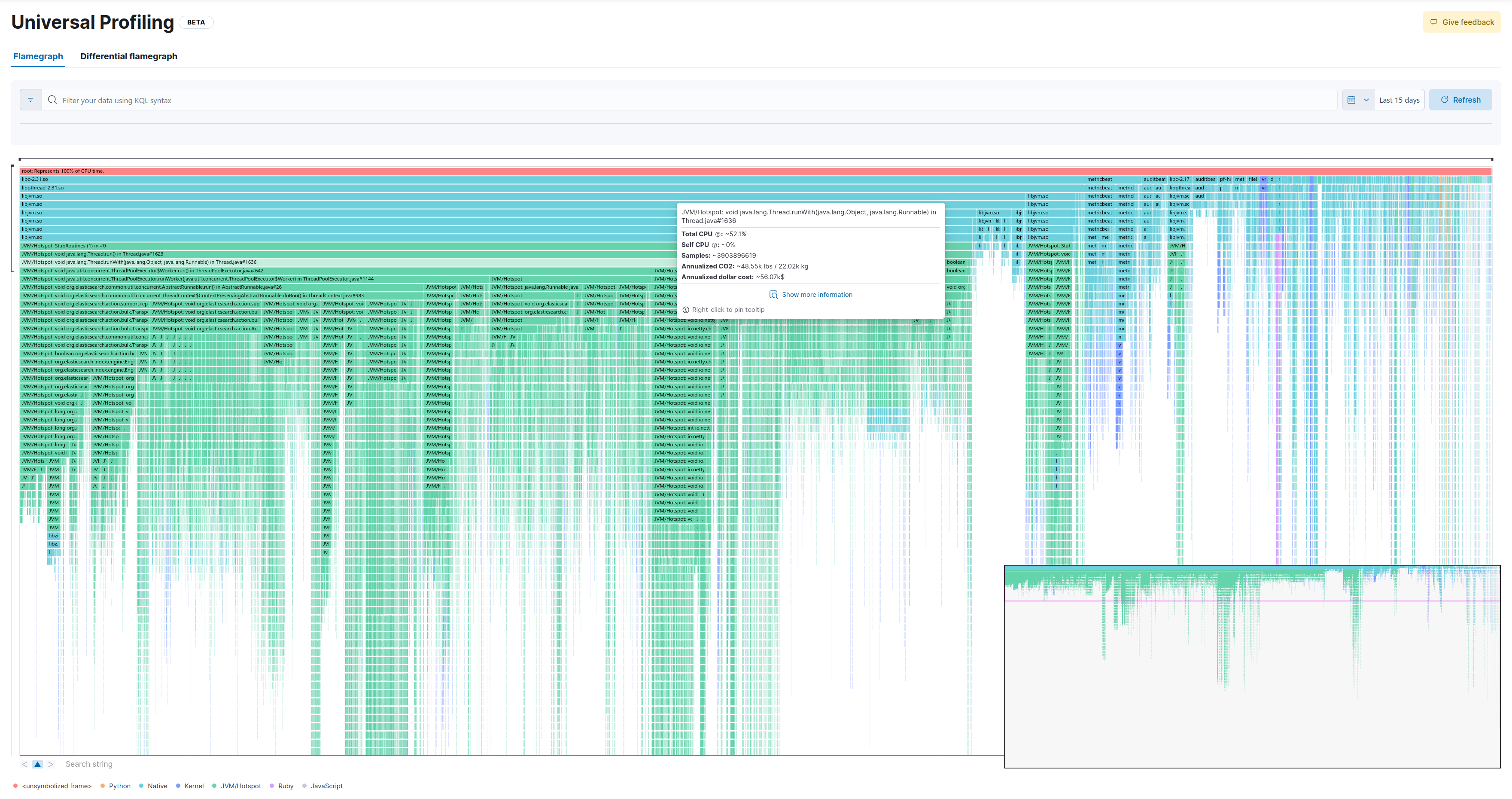
20.000 samples (1% distance)

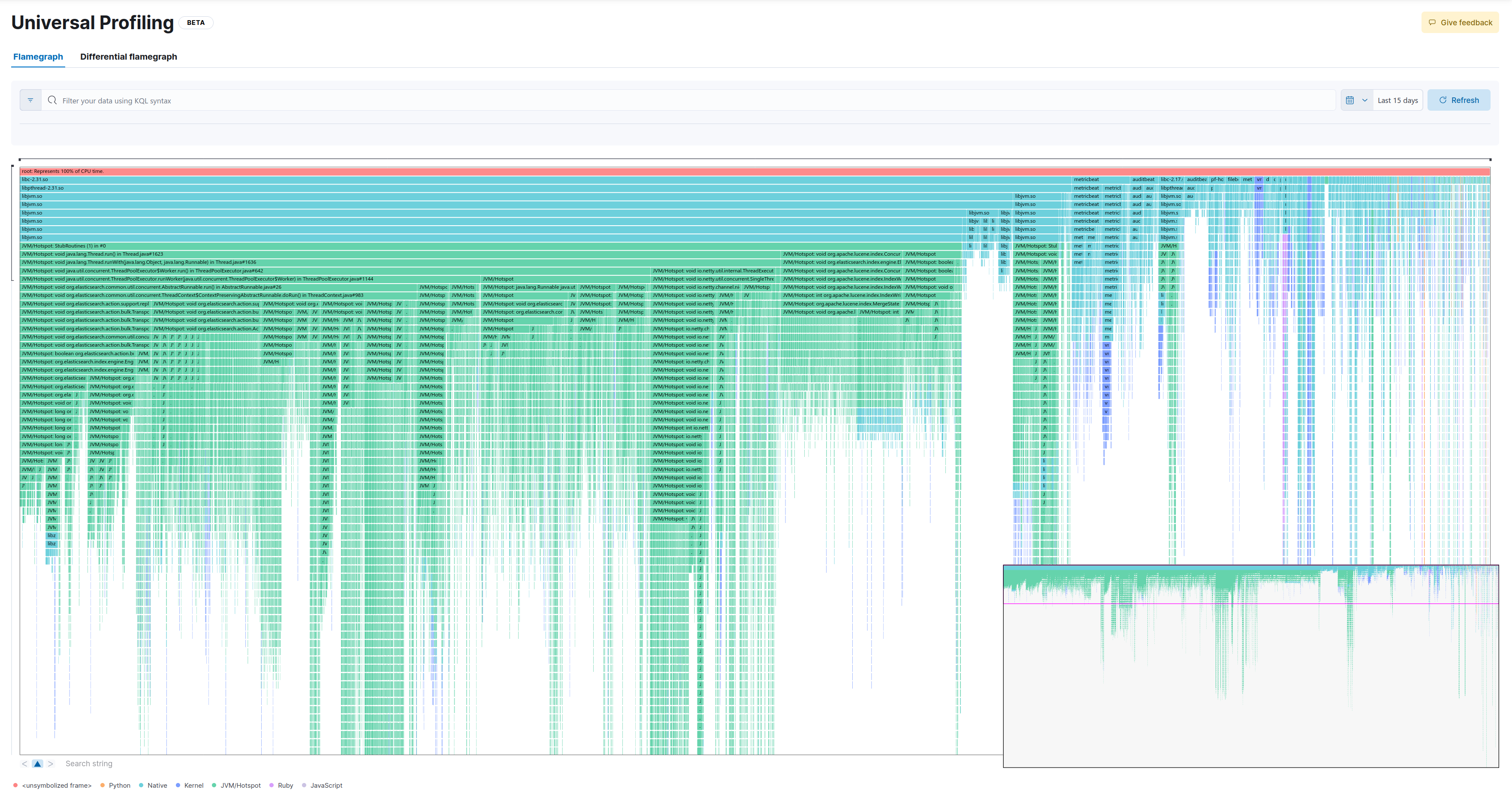
This is the full flamegraph:

Let’s zoom in a few levels. We’ll select the following method:

And this is how the respective flamegraph looks like:

4.925 samples (2% distance)

This is the full flamegraph:

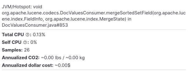
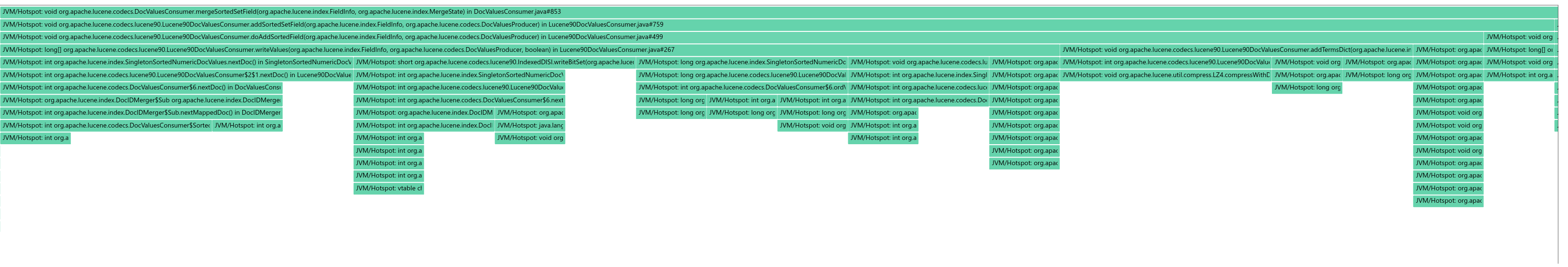
Now let’s drill down into the same method as in the baseline:

As we can see, we lose some samples which take up less CPU (in this example the widest stackframe at the top of the entire zoomed-in screen represents 26 samples). While this would probably not make much difference for most practical applications, there’s also a psychological component to it (Can I trust my profiler?).

The key problem is that stacktraces are not equally distributed but instead skewed heavily:

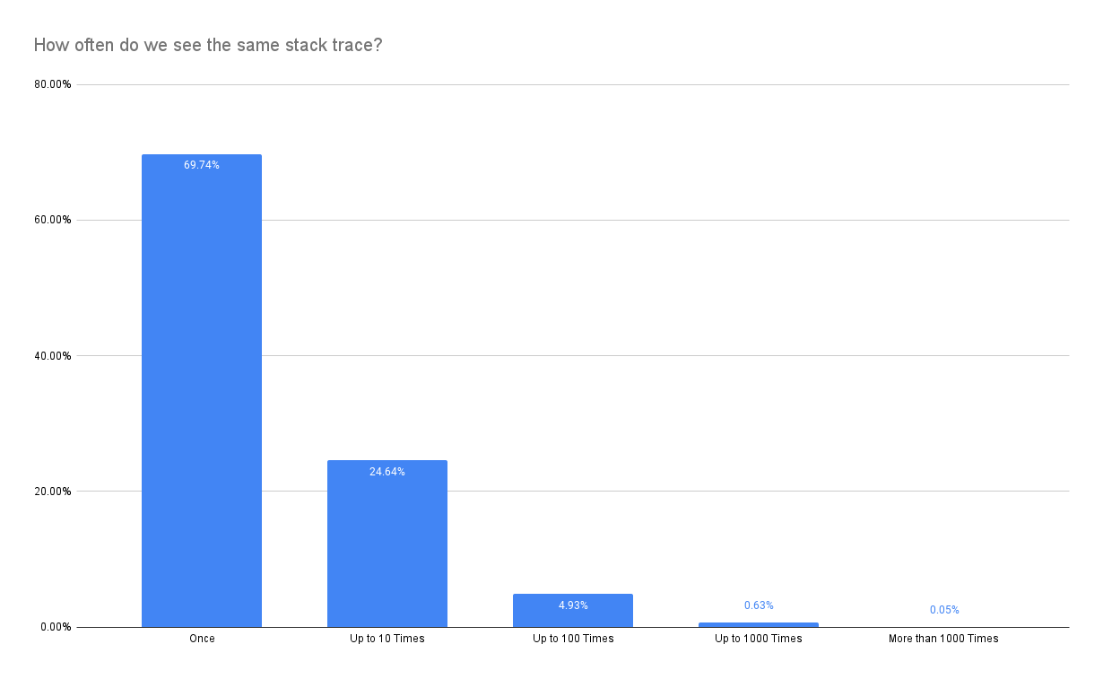
Therefore, it is much more likely that we eliminate one of the stacktraces that make up a spike (show up only once in the most extreme case) despite keeping the statistical properties promised by the sample size estimator. Nevertheless, relaxing constraints might still be a worthwhile option to reduce latency.