Daniel Mitterdorfer

When visualizing time series with more data points than available on-screen pixels we waste system resources and network bandwidth without adding any value. Therefore, various algorithms are available to reduce the data volume. One such algorithm is Largest-Triangle-Three-Buckets (LTTB) described by Sveinn Steinarsson in his master’s thesis. The key idea of the algorithm is to preserve the visual properties of the original data as much as possible by putting the original data in equally sized buckets and then determining the “most significant point” within each bucket. It does so by comparing adjacent points and selecting one point per bucket for which the largest triangle can be constructed (see page 19ff in the thesis for an in-depth description of the algorithm). The algorithm is implemented in various languages; in this blog post we’ll use the Python implementation in the lttb library.

Without any further ado, here is the algorithm in action downsampling an original data set consisting of 4096 samples to 1024 samples:

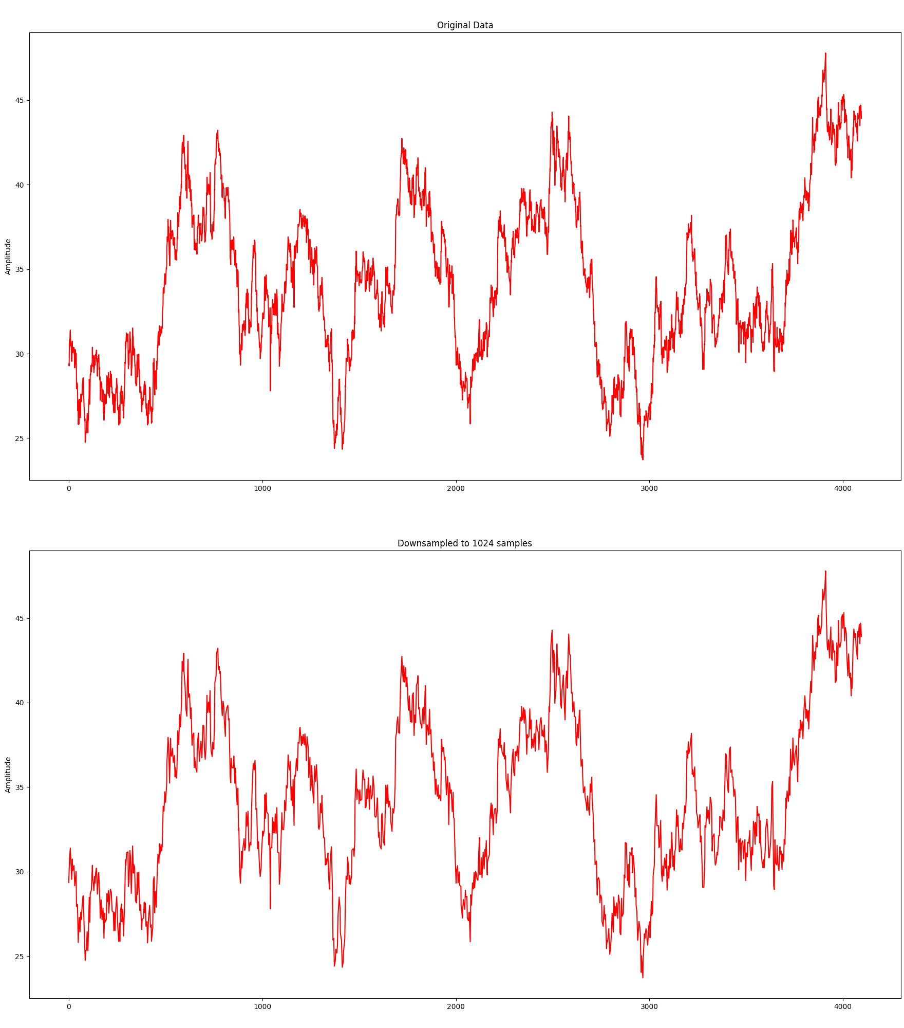
Although it needs only 25% of the samples, the visual representation is still relatively close. Let’s take it a bit further and try with 512 samples:

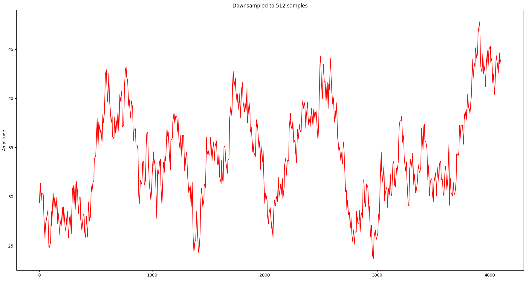
Although the overall shape is still relatively close, the information loss in local spikes starts to become noticeable.

From Time Domain to Frequency Domain: The Fourier Transform

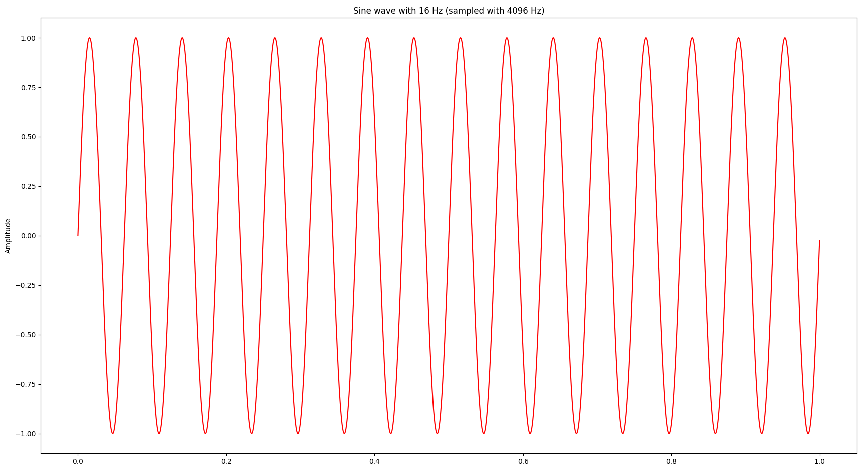
At this point I was wondering whether we can gain more insights by looking at the signal also in the frequency domain, which can be achieved by a Fourier transform. Bluntly speaking a Fourier transform decomposes a signal into a bunch of sine waves and provides the amplitude and frequency of each sine wave. Let’s start with a simple sine wave at 16 Hz (i.e. 16 oscillations per second):

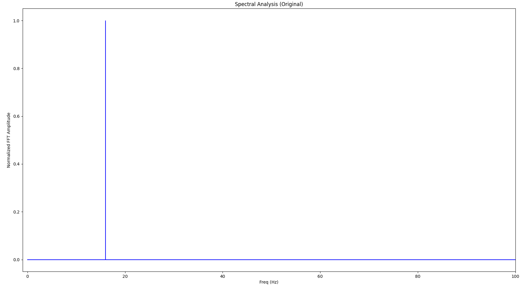
The Fourier transform looks as follows:

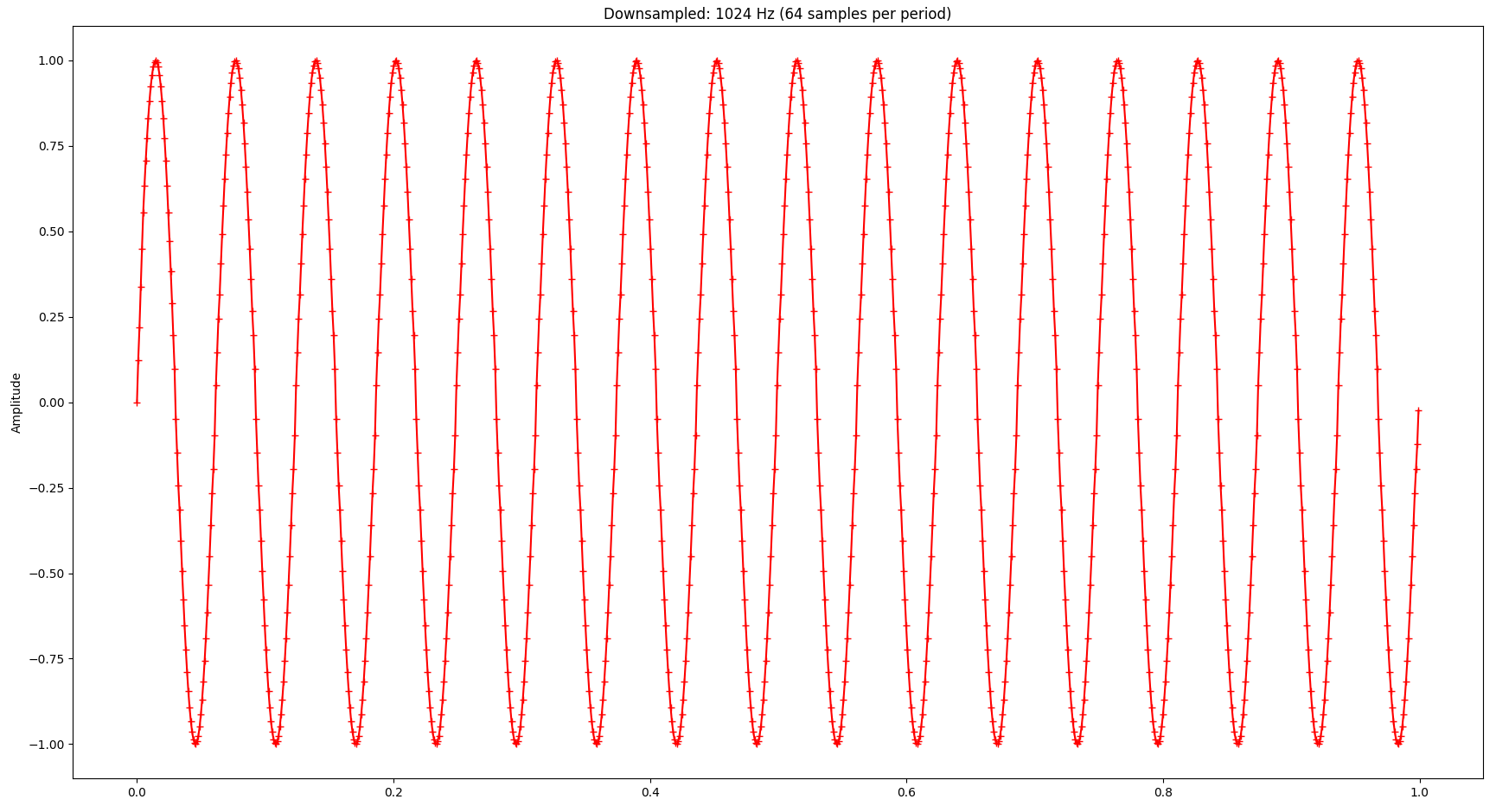
If we apply the LTTB algorithm to the sine wave and downsample it from the original 4096 points to 1024 points, the signal looks as follows (the little crosses indicate the samples picked by LTTB):

And the Fourier transform looks as follows:

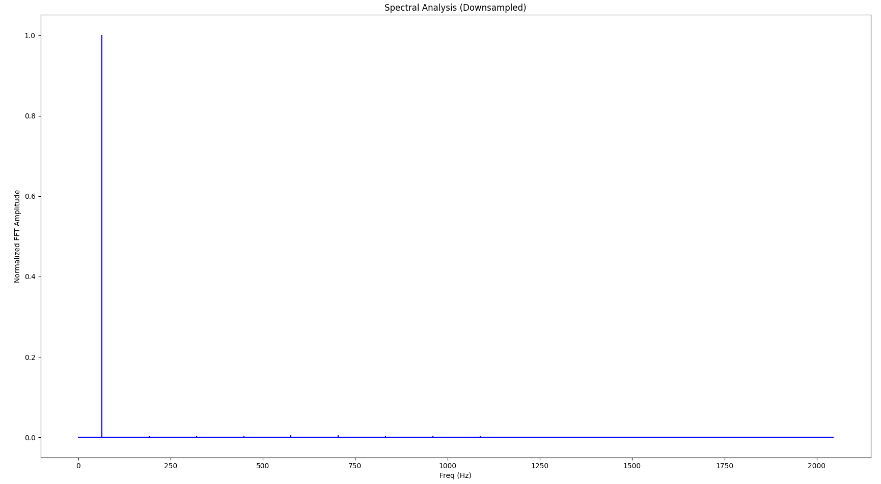
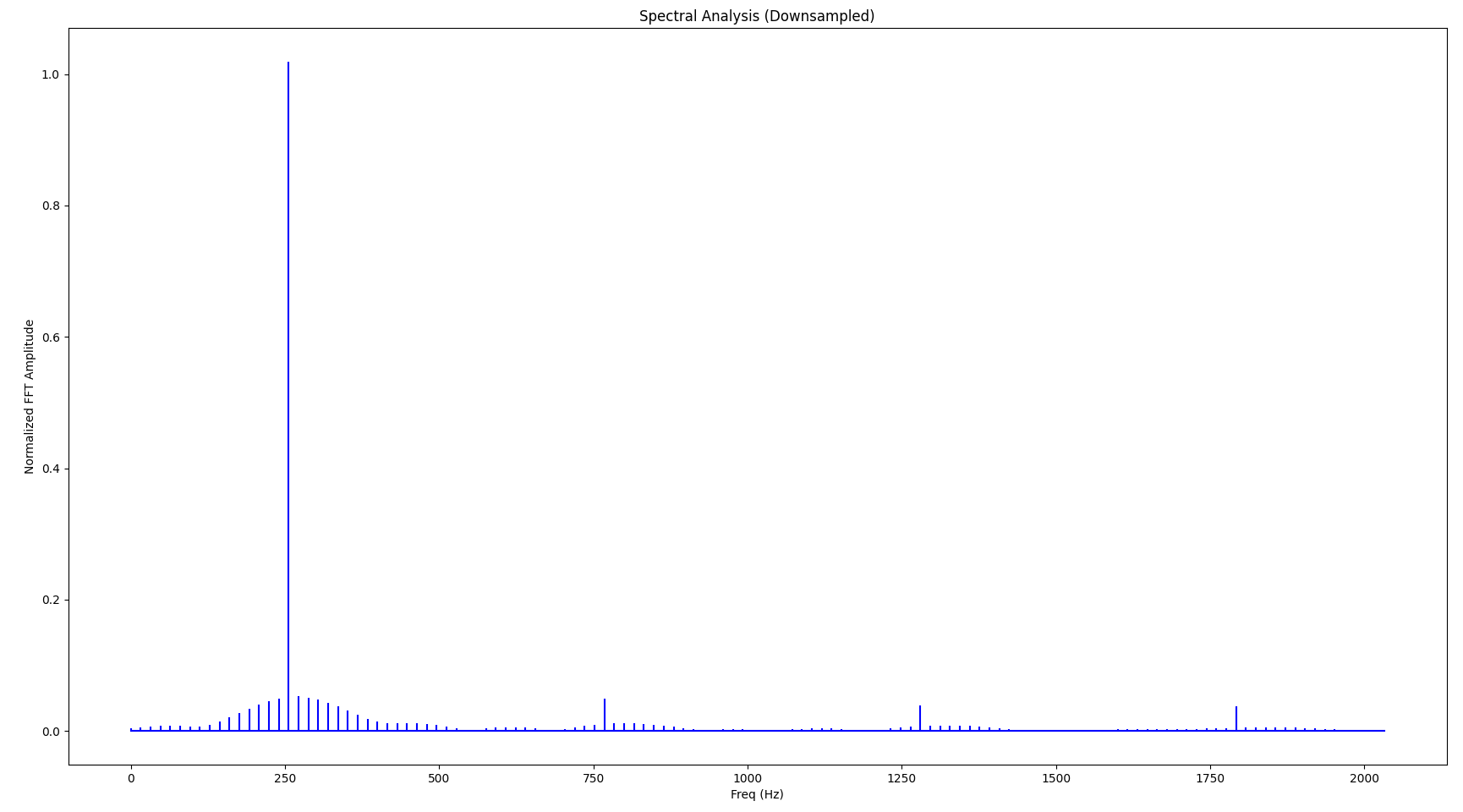
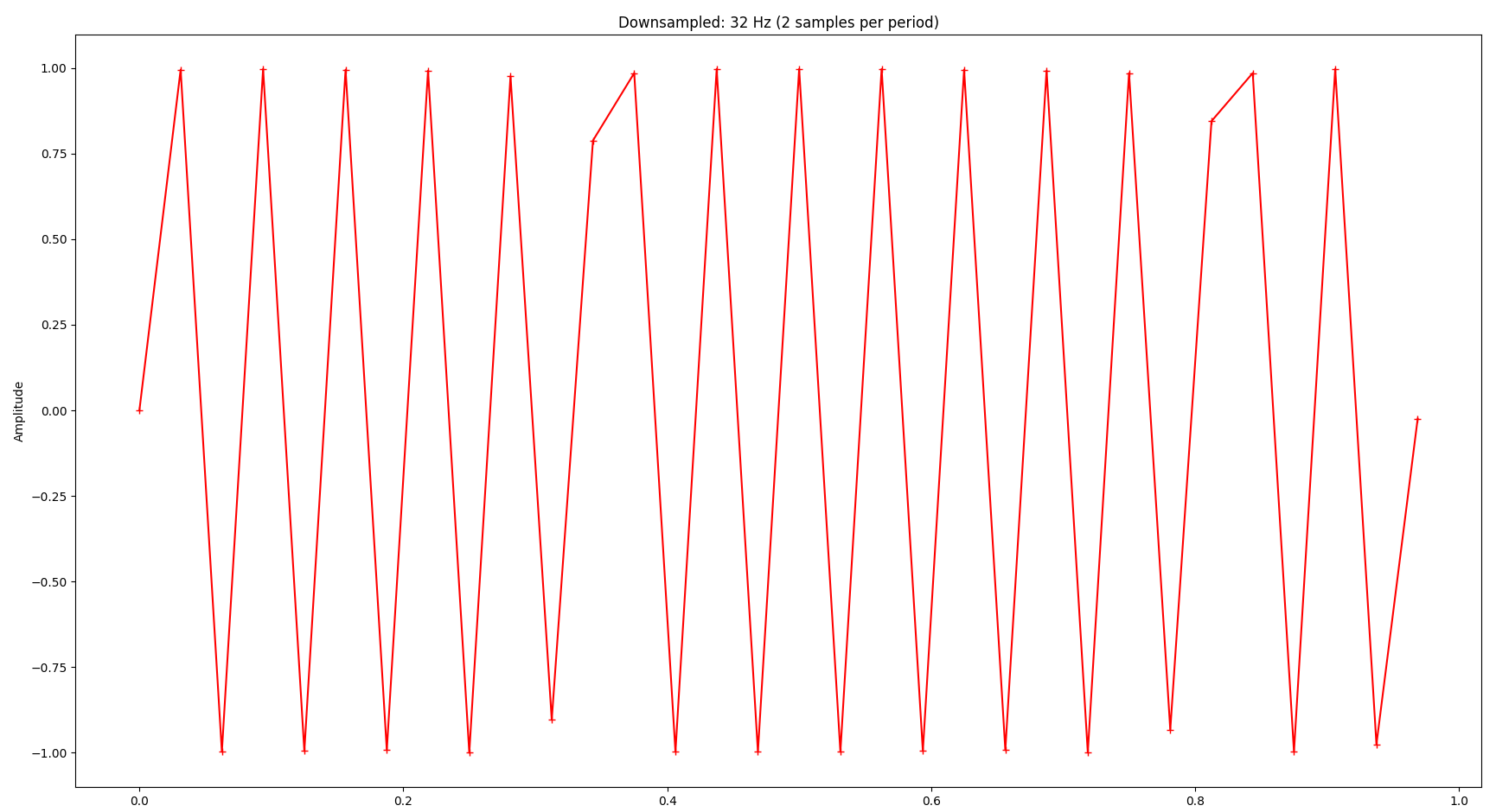
If you look closely, you’ll notice that the base frequency (the largest spike in the spectrum) is not 16 Hz but 32 Hz, also there are a few very small spikes at higher frequencies (“harmonic waves”). These distortion artifacts in the frequency domain are caused by the downsampling. As we continue to downsample more aggressively, the signal gets worse both in the time domain and the frequency domain. Also, as we lower the sampling frequency, the resulting signal’s base frequency increases accordingly. The following diagrams show the same signal but with only 256 samples:

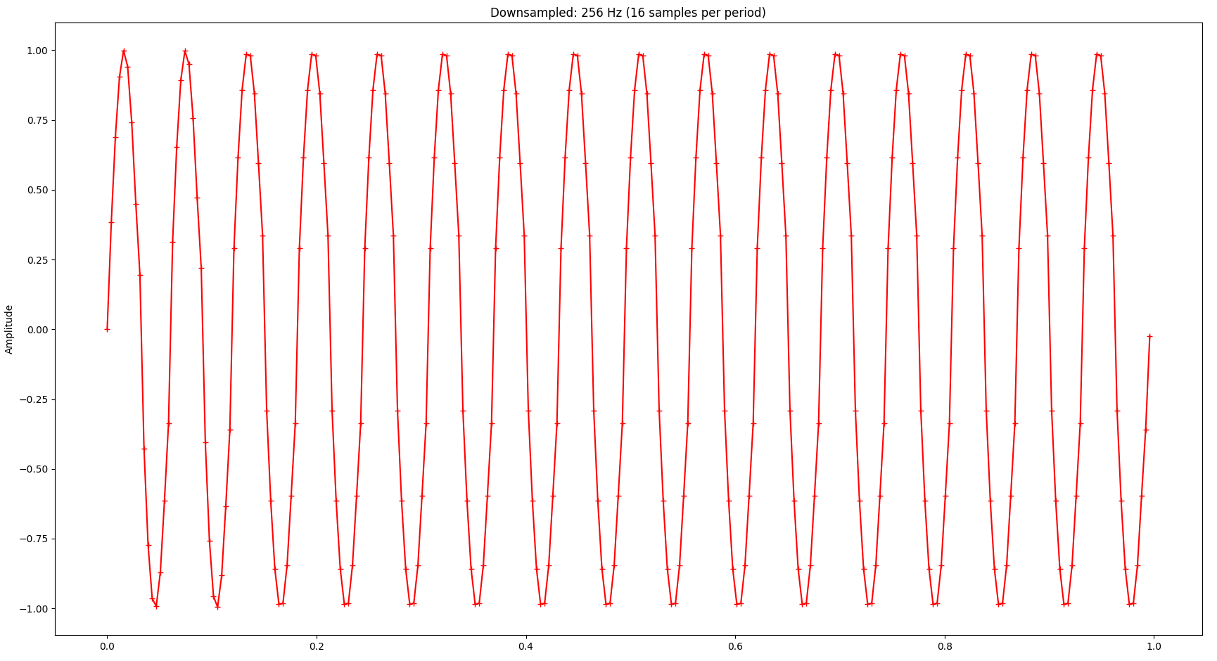
While the visual representation is still relatively ok - considering that we only kept 6.25% of the original samples - we notice relatively serious distortion in the frequency domain. Also notice how the base frequency (largest spike) changed to 256 Hz:

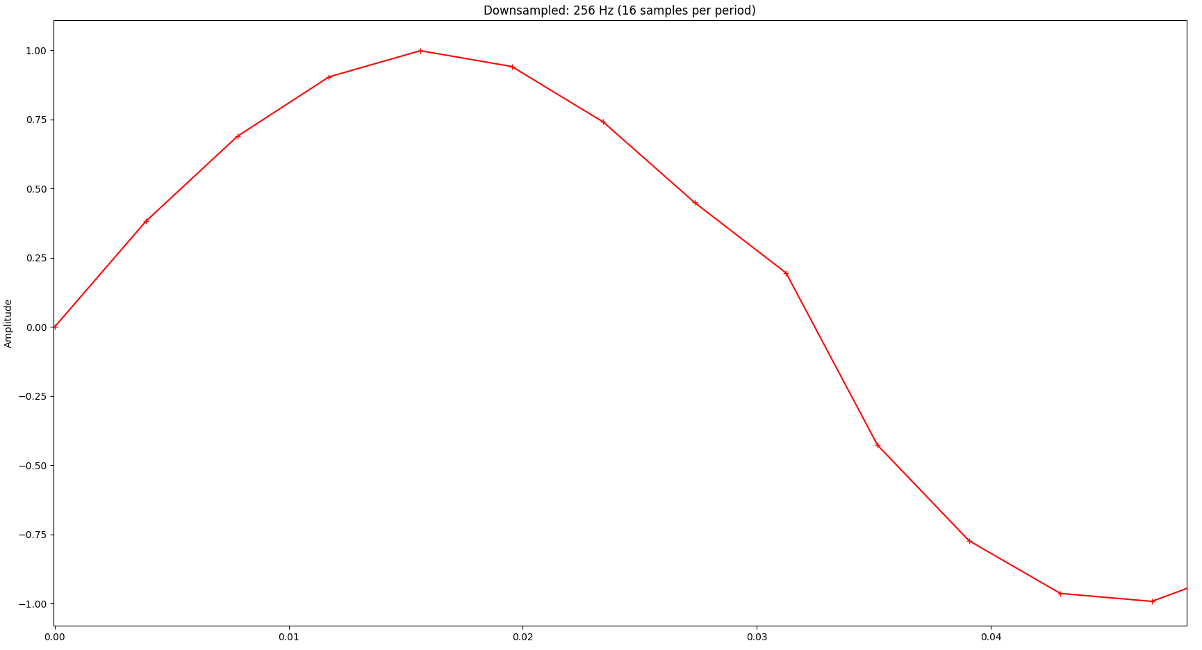
Also, a close-up to just one period of the signal reveals quite significant distortion:

Exploring Boundaries

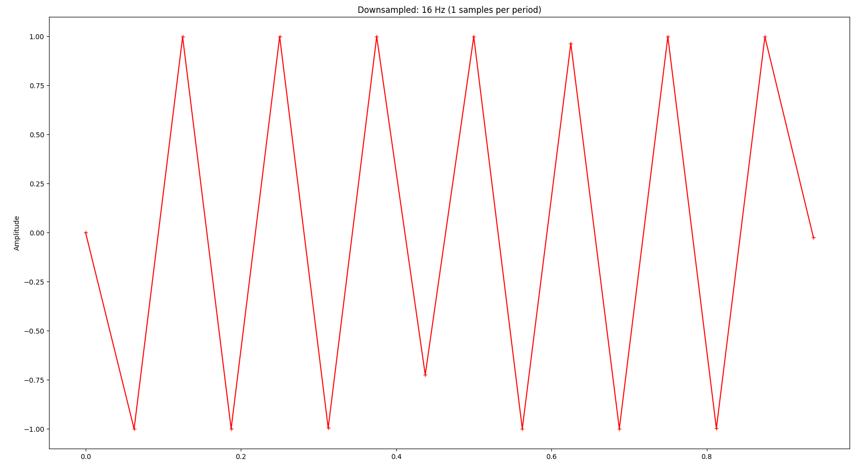
Now you might wonder: How far can we reduce the sampling rate? The Nyquist–Shannon sampling theorem basically states that we need to sample at least at two times the highest frequency in the signal we’re interested in. In our example that frequency is 16 Hz, so the sampling frequency should be at least 2 * 16 Hz = 32 Hz. As you can see, we can still infer the original signal’s frequency at 32 samples:

The signal is completely distorted if we go below that:

Application to the Original Signal

Now let’s apply that knowledge to our original signal, which is more complicated. The FFT of the original signal looks as follows. The vertical gray lines indicate 16 Hz, 32 Hz and 48 Hz respectively.

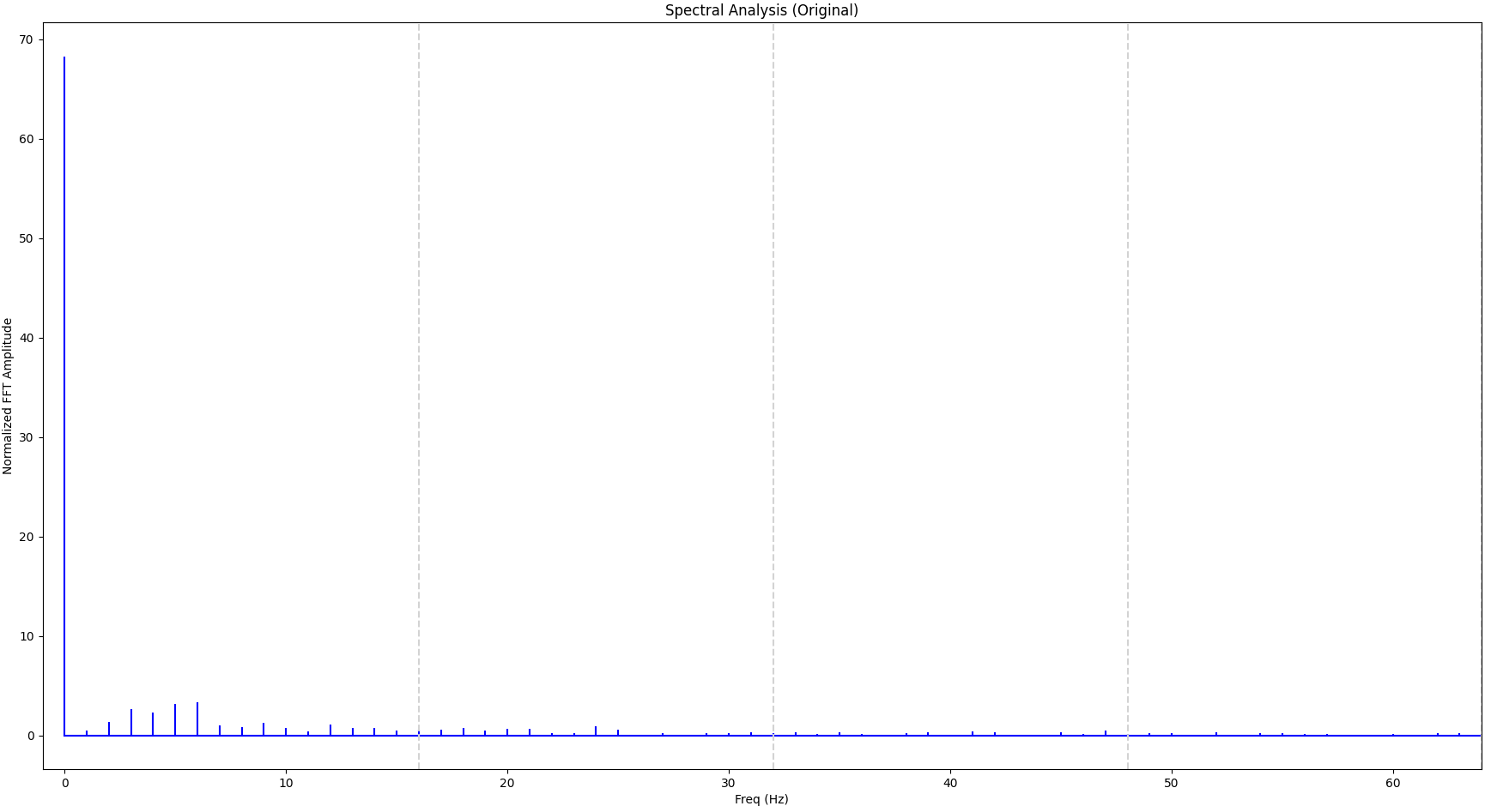
We can see that a significant portion of the signal is within the first 16 Hz bucket so we can attempt with 32 samples. For comparison we will also sample with just 8 samples. The result is shown below, together with the original signal:

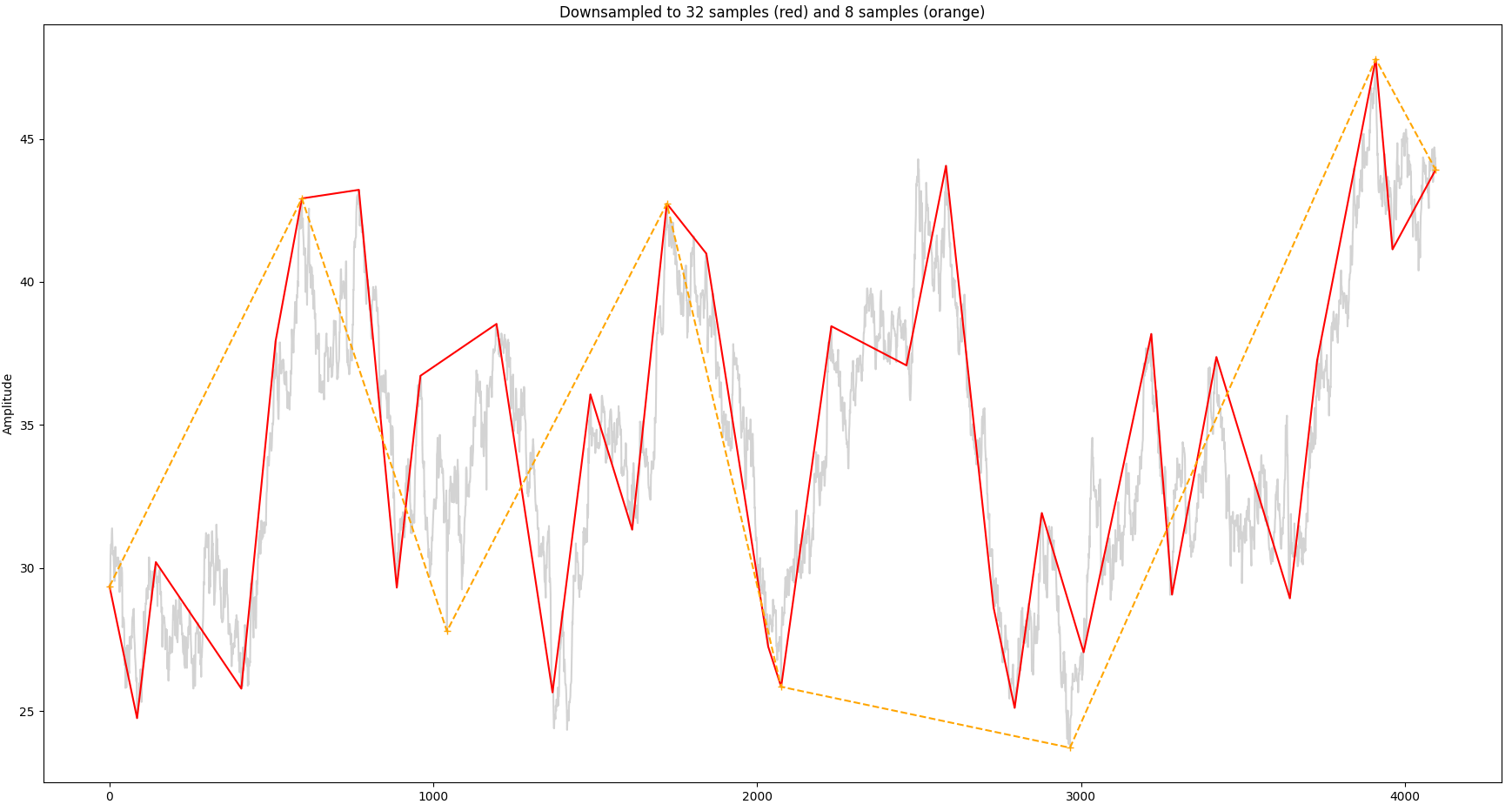
So the overall shape of the signal is still recognizable with 32 samples as opposed to just 8 samples.

Summary

Downsampling saves system resources and improves rendering latency. The Largest-Triangle-Three-Buckets (LTTB) algorithm is specifically geared towards preserving visual properties. In this blog post we have applied concepts from signal processing such Fourier transform to explore boundaries when parameterizing this algorithm and discussed the Nyquist theorem.