Recent Posts
Largest-Triangle-Three-Buckets and the Fourier Transform
Written on Tue, Jan 30, 2024
When visualizing time series with more data points than available on-screen pixels we waste system resources and network bandwidth without adding any value. Therefore, various algorithms are available to reduce the data volume. One such algorithm is Largest-Triangle-Three-Buckets (LTTB) described by Sveinn Steinarsson in his master’s thesis. The key idea of the algorithm is to preserve the visual properties of the original data as much as possible by putting the original data in equally sized buckets and then determining the “most significant point” within each bucket. It does so by comparing adjacent points and selecting one point per bucket for which the largest triangle can be constructed (see page 19ff in the thesis for an in-depth description of the algorithm). The algorithm is implemented in various languages; in this blog post we’ll use the Python implementation in the lttb library.
Without any further ado, here is the algorithm in action downsampling an original data set consisting of 4096 samples to 1024 samples:
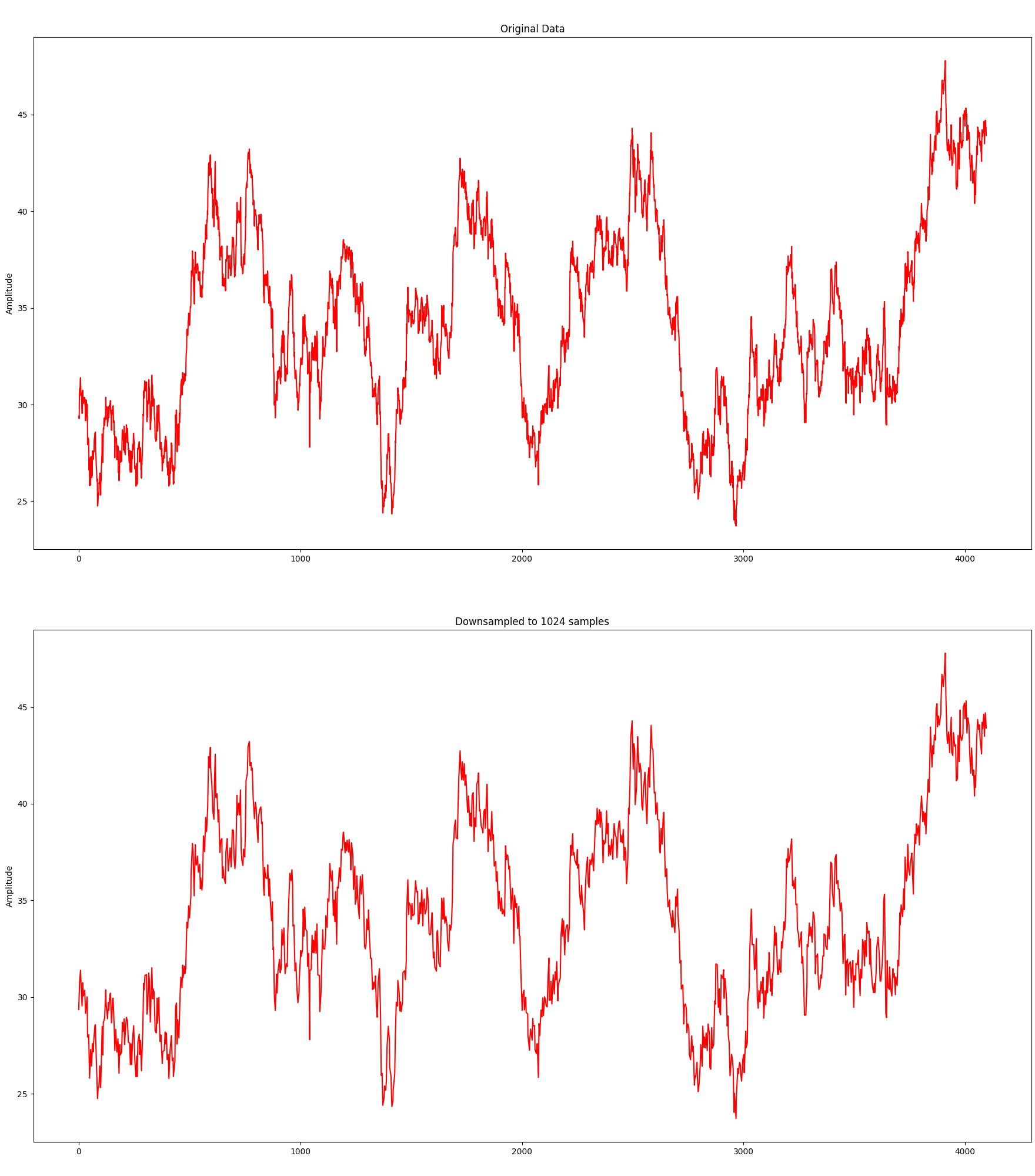
Although it needs only 25% of the samples, the visual representation is still relatively close. Let’s take it a bit further and try with 512 samples:
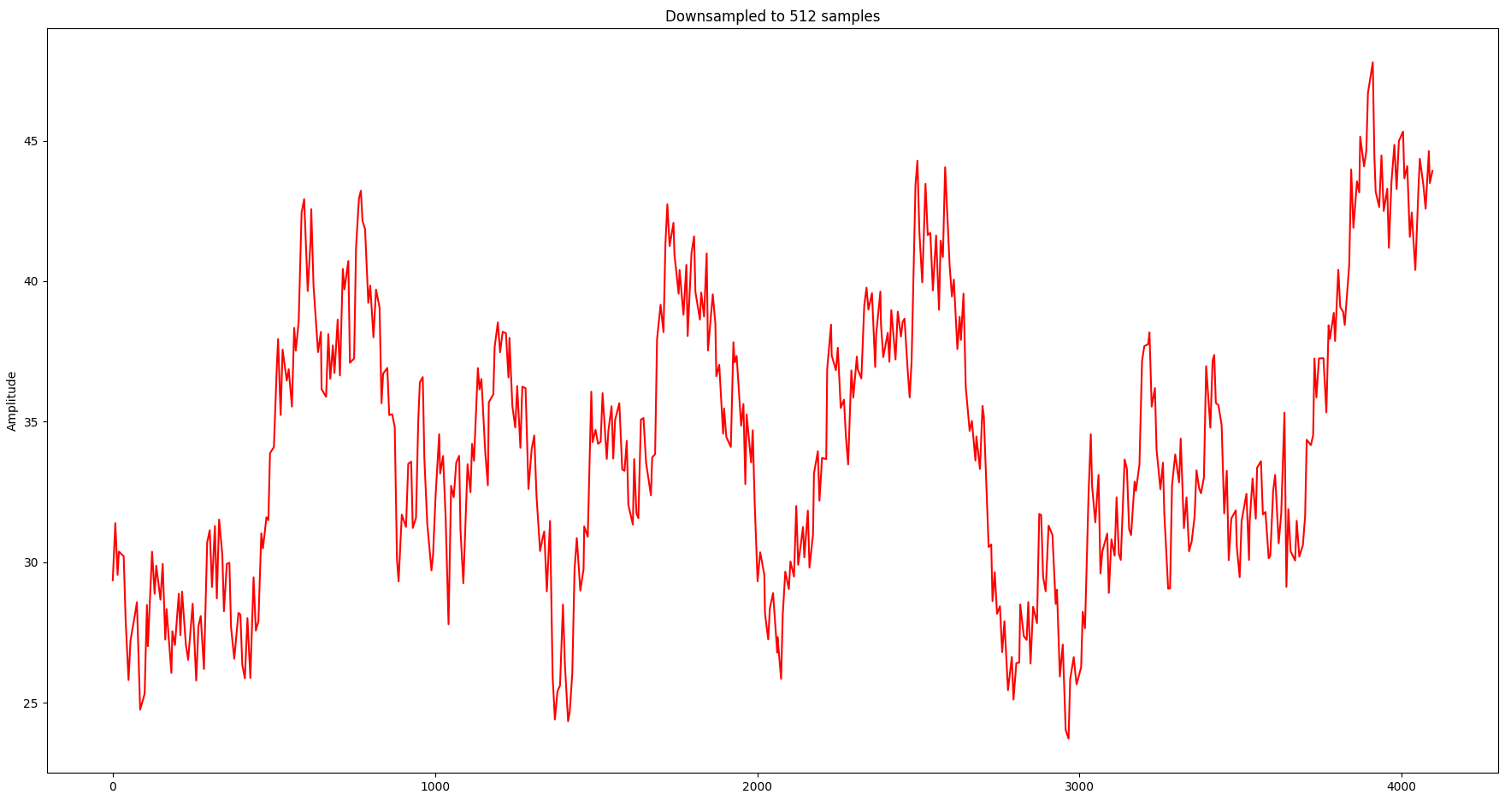
Although the overall shape is still relatively close, the information loss in local spikes starts to become noticeable.
From Time Domain to Frequency Domain: The Fourier Transform
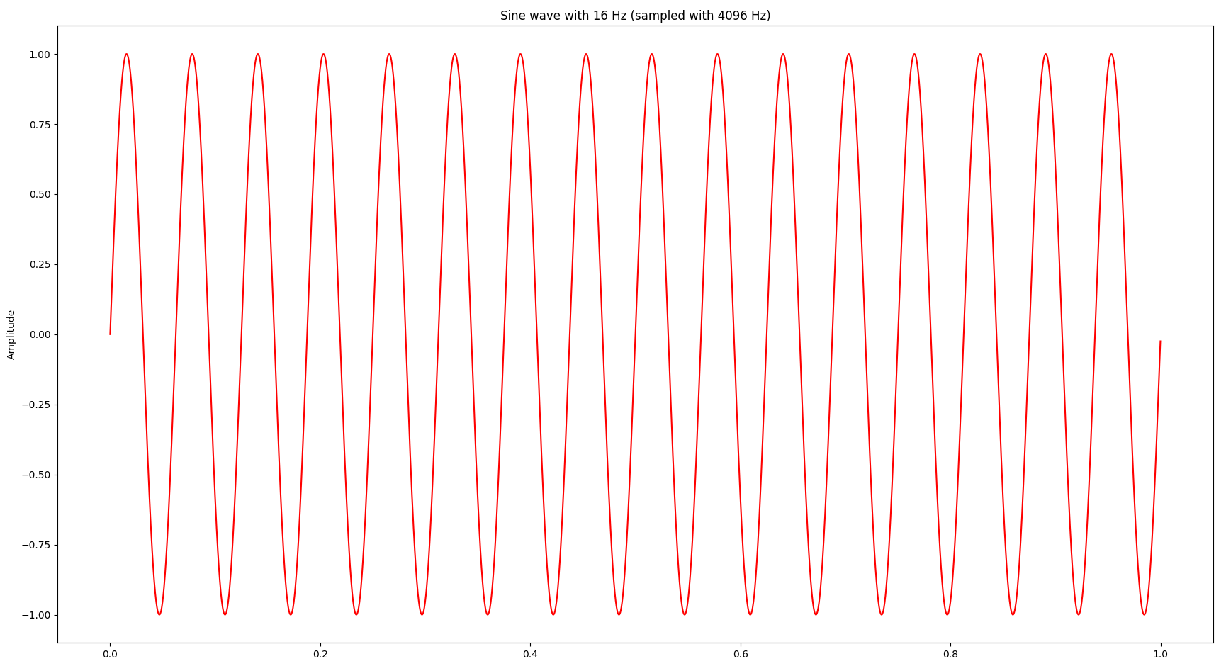
At this point I was wondering whether we can gain more insights by looking at the signal also in the frequency domain, which can be achieved by a Fourier transform. Bluntly speaking a Fourier transform decomposes a signal into a bunch of sine waves and provides the amplitude and frequency of each sine wave. Let’s start with a simple sine wave at 16 Hz (i.e. 16 oscillations per second):
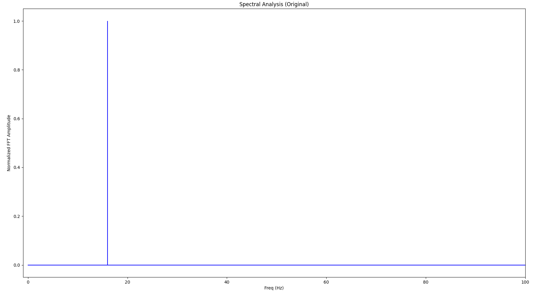
The Fourier transform looks as follows:
If we apply the LTTB algorithm to the sine wave and downsample it from the original 4096 points to 1024 points, the signal looks as follows (the little crosses indicate the samples picked by LTTB):
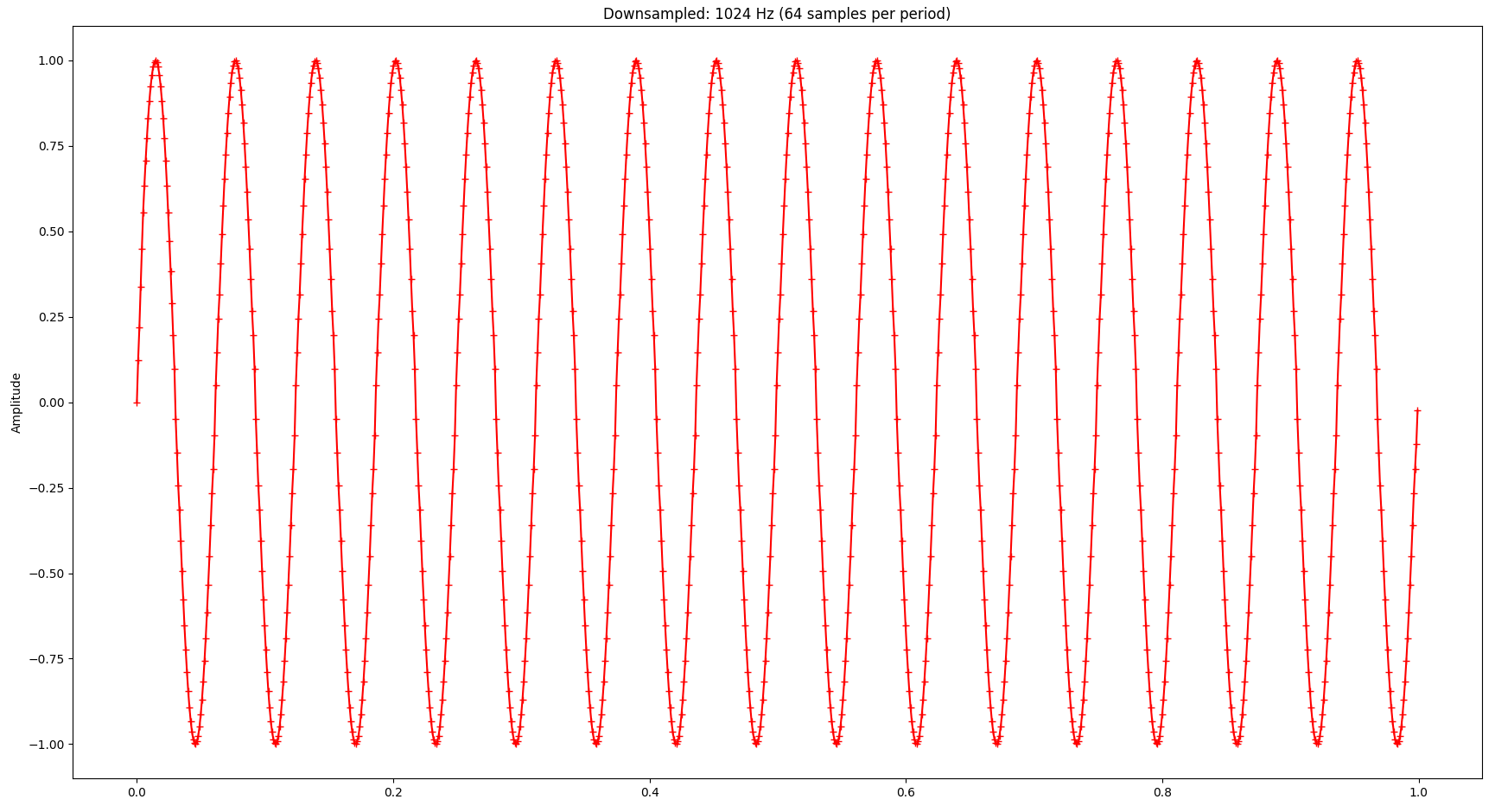
And the Fourier transform looks as follows:
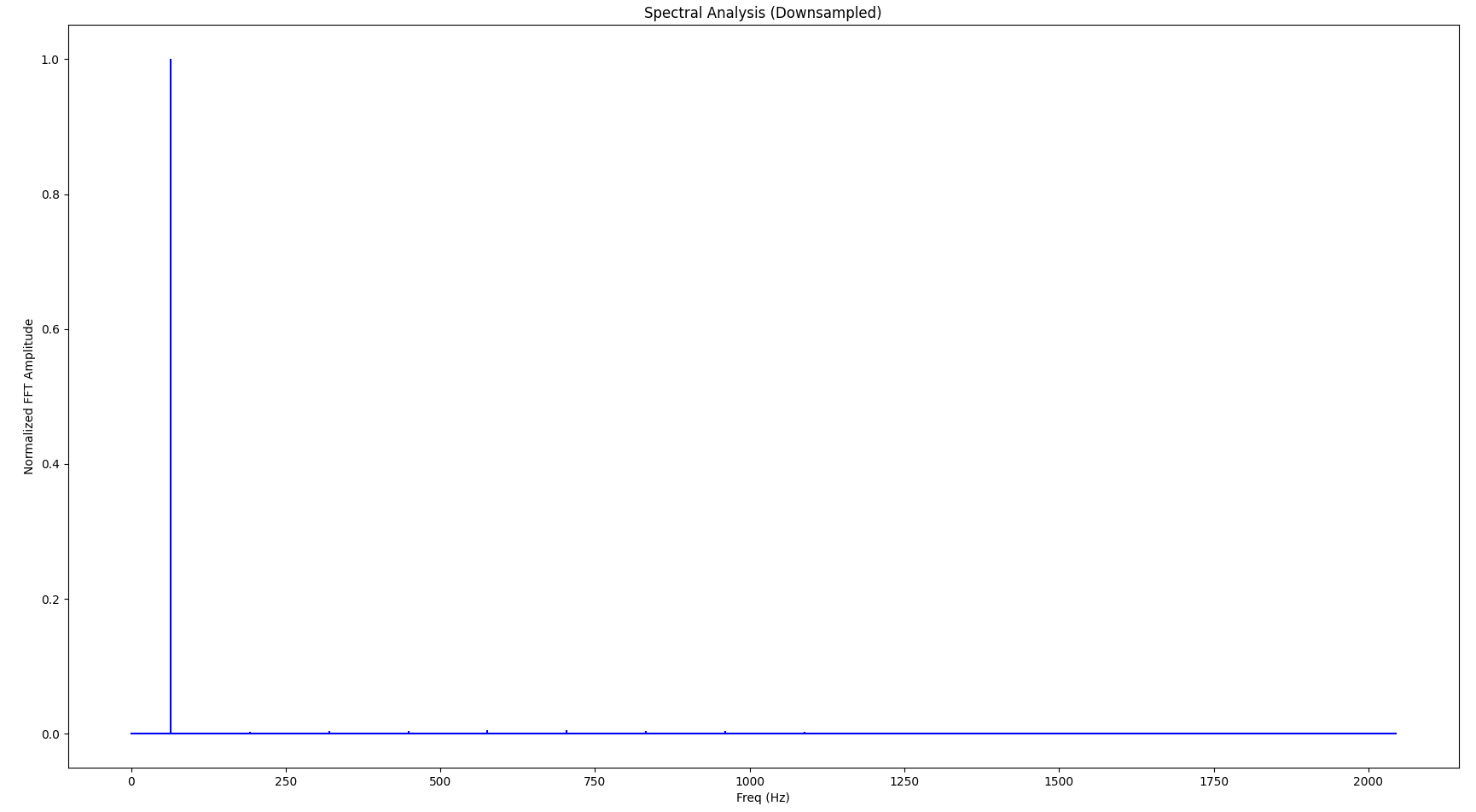
If you look closely, you’ll notice that the base frequency (the largest spike in the spectrum) is not 16 Hz but 32 Hz, also there are a few very small spikes at higher frequencies (“harmonic waves”). These distortion artifacts in the frequency domain are caused by the downsampling. As we continue to downsample more aggressively, the signal gets worse both in the time domain and the frequency domain. Also, as we lower the sampling frequency, the resulting signal’s base frequency increases accordingly. The following diagrams show the same signal but with only 256 samples:
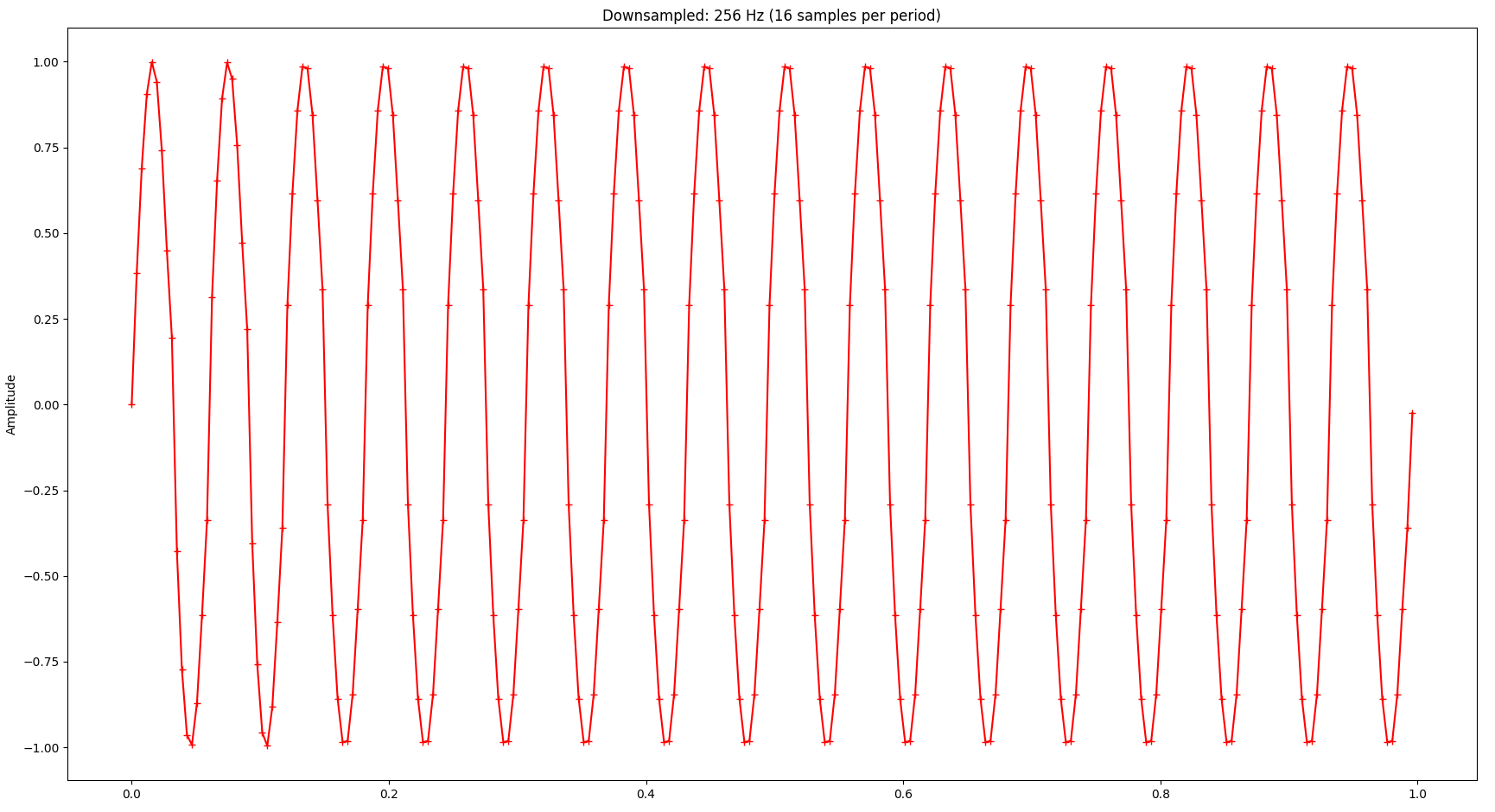
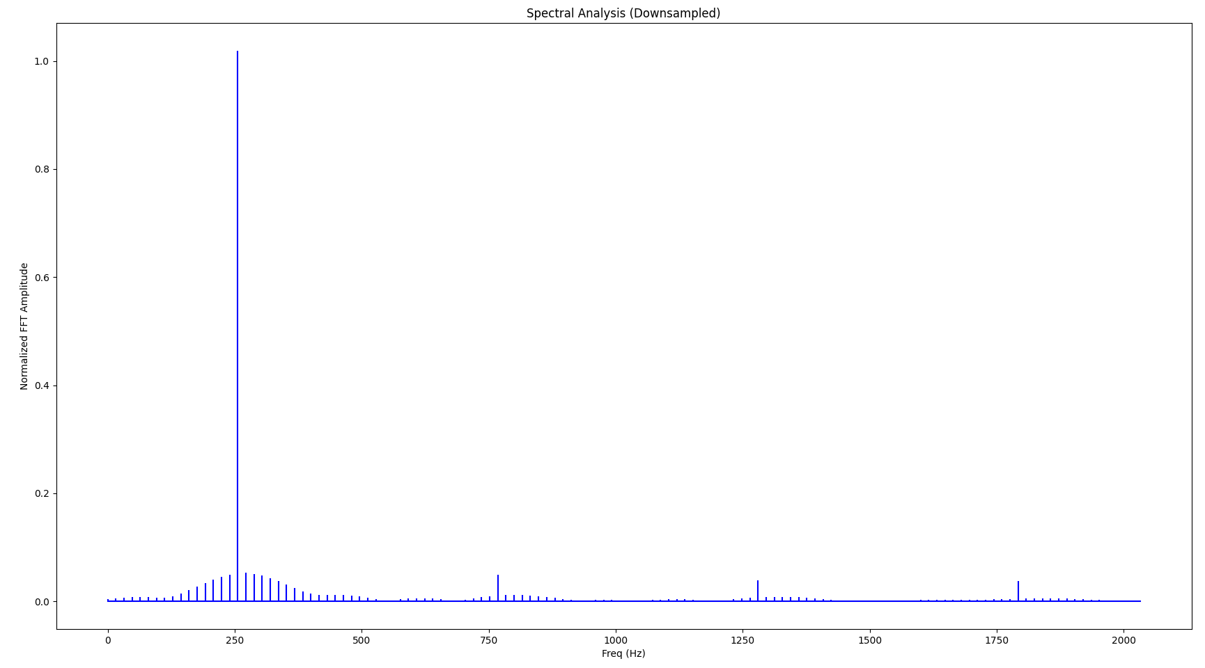
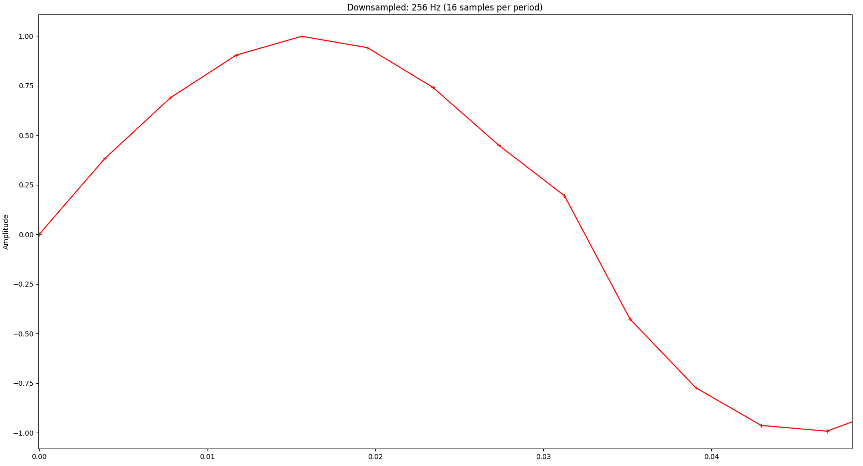
While the visual representation is still relatively ok - considering that we only kept 6.25% of the original samples - we notice relatively serious distortion in the frequency domain. Also notice how the base frequency (largest spike) changed to 256 Hz:
Also, a close-up to just one period of the signal reveals quite significant distortion:
Exploring Boundaries
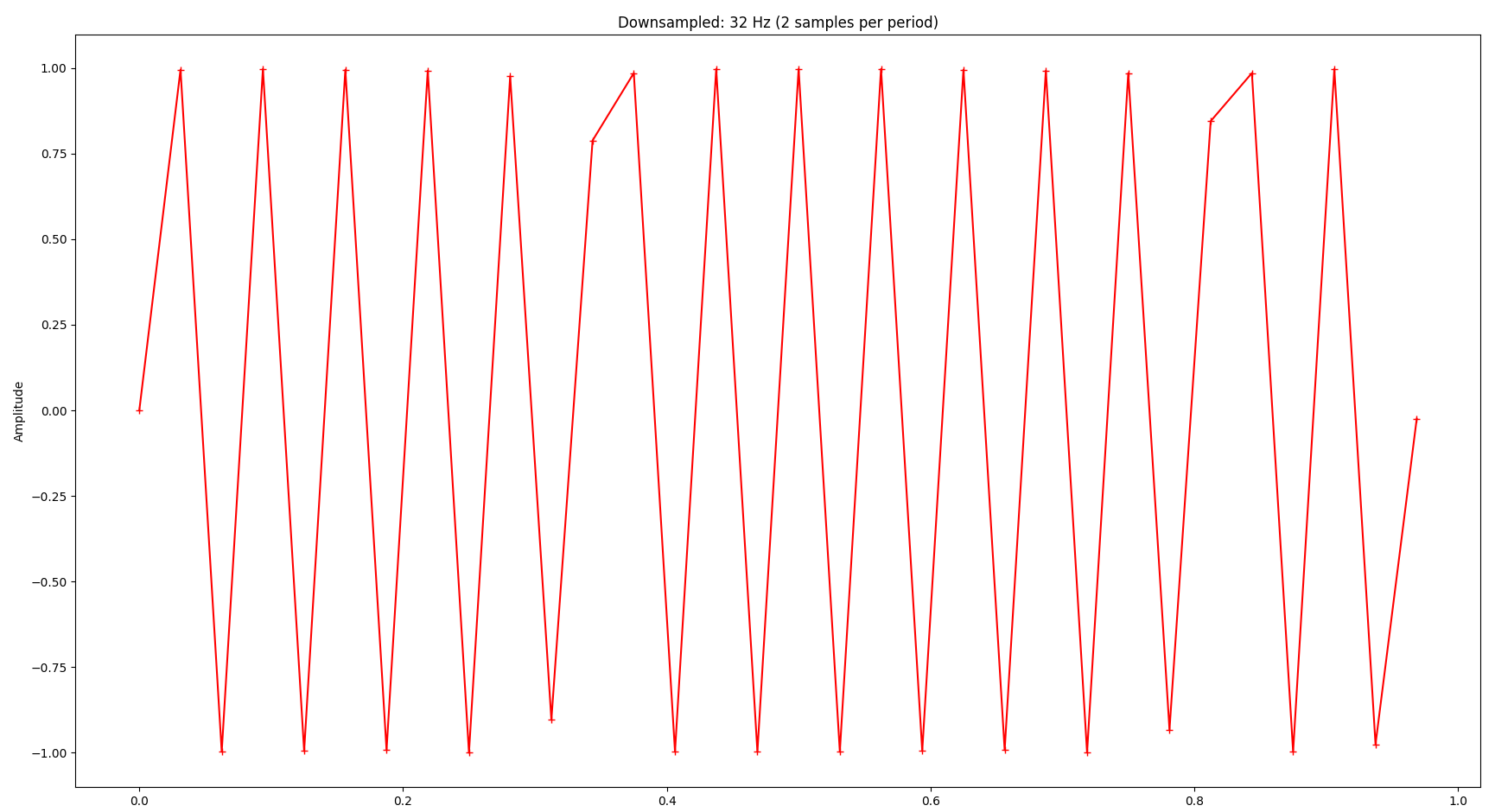
Now you might wonder: How far can we reduce the sampling rate? The Nyquist–Shannon sampling theorem basically states that we need to sample at least at two times the highest frequency in the signal we’re interested in. In our example that frequency is 16 Hz, so the sampling frequency should be at least 2 * 16 Hz = 32 Hz. As you can see, we can still infer the original signal’s frequency at 32 samples:
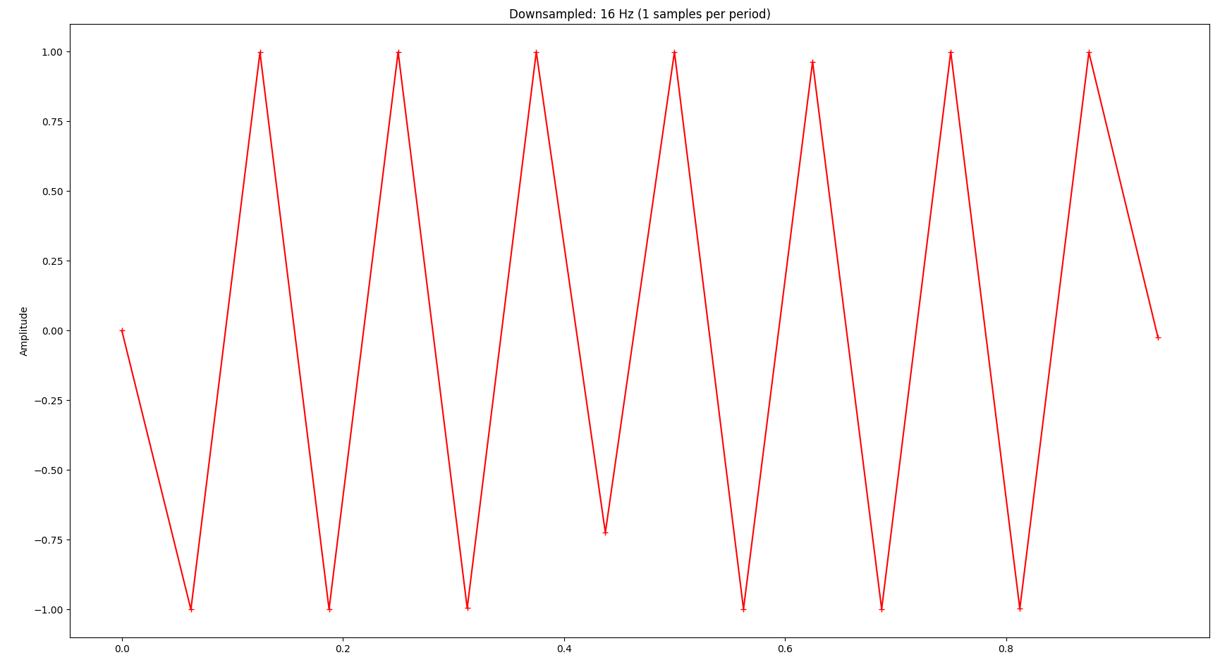
The signal is completely distorted if we go below that:
Application to the Original Signal
Now let’s apply that knowledge to our original signal, which is more complicated. The FFT of the original signal looks as follows. The vertical gray lines indicate 16 Hz, 32 Hz and 48 Hz respectively.
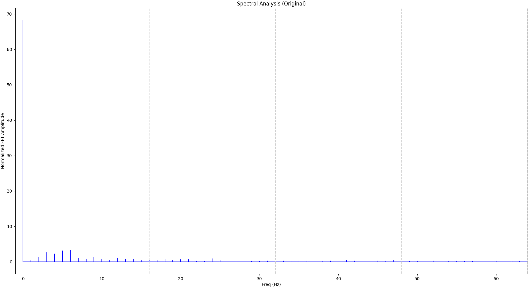
We can see that a significant portion of the signal is within the first 16 Hz bucket so we can attempt with 32 samples. For comparison we will also sample with just 8 samples. The result is shown below, together with the original signal:
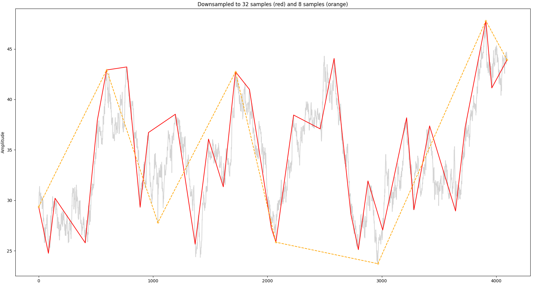
So the overall shape of the signal is still recognizable with 32 samples as opposed to just 8 samples.
Summary
Downsampling saves system resources and improves rendering latency. The Largest-Triangle-Three-Buckets (LTTB) algorithm is specifically geared towards preserving visual properties. In this blog post we have applied concepts from signal processing such Fourier transform to explore boundaries when parameterizing this algorithm and discussed the Nyquist theorem.
Latency Analysis of Elasticsearch
Written on Sun, Oct 15, 2023
I currently work on the backend of Elastic Universal Profiling, which is a fleet-wide continuous profiler. In our benchmarks we have observed higher than desired latency in a query that retrieves data for flamegraphs. As this is a key aspect of our product we wanted to better understand the root cause.
CPU Profiling
We started to gather CPU profiles with async-profiler in Wall-clock profiling mode on the Elasticsearch cluster while it was processing a query:
The diagram above shows an activity timeline for one of the threads involved in query processing.The thread is only active for a brief period of time around the middle of the timeline but is otherwise idle. Other involved threads show a similar pattern. In other words, this query is not CPU bound. We therefore analyzed disk utilization but also disk I/O was far below the supported IOPS. So if the problem is neither the time spent on CPU nor disk I/O, what should we do to get to the bottom of this mystery?
Off-CPU Analysis
Time for off-CPU analysis! Put bluntly, we want to see why the CPU is not doing anything. We will use perf sched record to do this. Around the time the query is executed, we’ll run the following command:
perf sched record -g -- sleep $PROFILING_DURATION
This traces CPU scheduler events and creates a perf.data file that we can analyze, e.g. using perf sched timehist -V. The data in this file tell us when, for how long and why a thread went off-CPU (slightly edited for brevity):
           time task name                       wait time  sch delay   run time
                [tid/pid]                          (msec)     (msec)     (msec)
--------------- ------------------------------  ---------  ---------  ---------
   15589.656599 elasticsearch[e[8937/8881]          0.000      0.000      0.020    [unknown] <- [unknown] <- [unknown] <- [...]
   15589.656601 Attach Listener[9157/8881]          0.162      0.000      0.053    [unknown] <- [unknown] <- [unknown] <- [...]
   15589.656601 <idle>                              0.023      0.000      0.231
   15589.656605 elasticsearch[e[8936/8881]          0.000      0.000      0.022    [unknown] <- [unknown] <- [unknown] <- [...]
   15589.656609 <idle>                              0.009      0.000      0.433
   15589.656616 elasticsearch[d[8953/8881]          0.000      0.000      0.014    [unknown] <- [unknown] <- [unknown] <- [...]
   15589.656623 elasticsearch[e[8956/8881]          0.000      0.000      0.014    [unknown] <- [unknown] <- [unknown] <- [...]
   15589.656753 <idle>                              0.053      0.000      0.152
   15589.656762 <idle>                              0.015      0.000      0.389
   15589.656765 <idle>                              0.015      0.000      0.173
That doesn’t look too useful because kernel symbols are missing. So make sure to install them first (check your distro’s docs how to do this). If kernel symbols are available, the output looks as follows (slightly edited for brevity):
         time task name                   wait time  sch delay   run time
              [tid/pid]                      (msec)     (msec)     (msec)
------------- --------------------------  ---------  ---------  ---------
 17452.955493 <idle>                          0.165      0.000      0.018
 17452.955494 elasticsearch[i[9782/8239]      0.000      0.000      0.044    futex_wait_queue_me <- futex_wait <- do_futex <- __x64_sys_futex
 17452.955507 elasticsearch[i[9388/8239]      0.000      0.000      0.036    futex_wait_queue_me <- futex_wait <- do_futex <- __x64_sys_futex
 17452.955509 <idle>                          0.041      0.000      0.464
 17452.955639 <idle>                          0.068      0.000      0.168
 17452.955682 <idle>                          0.027      0.000      0.208
 17452.955684 <idle>                          0.021      0.000      0.194
 17452.955687 <idle>                          0.024      0.000      0.170
 17452.955689 elasticsearch[i[5892/4393]      0.558      0.000      0.180    io_schedule <- __lock_page_killable <- filemap_fault <- __xfs_filemap_fault
That’s much better. Looking at the last line in the output, we can infer that an Elasticsearch thread was running for 180µs and was then blocked for 558µs because it caused a page fault. While this is useful, our ultimate goal is to analyze and eliminate major latency contributors. Just looking at this output does not help us understand what piece of code in the application has caused that page fault. Ideally we’d like to see the off-CPU profile integrated with the on-CPU profile. Then we’d be able to see what piece of code has caused the application to block and what it is blocked on (e.g. page fault handling, locking, blocking disk I/O).
Combining both Profiles
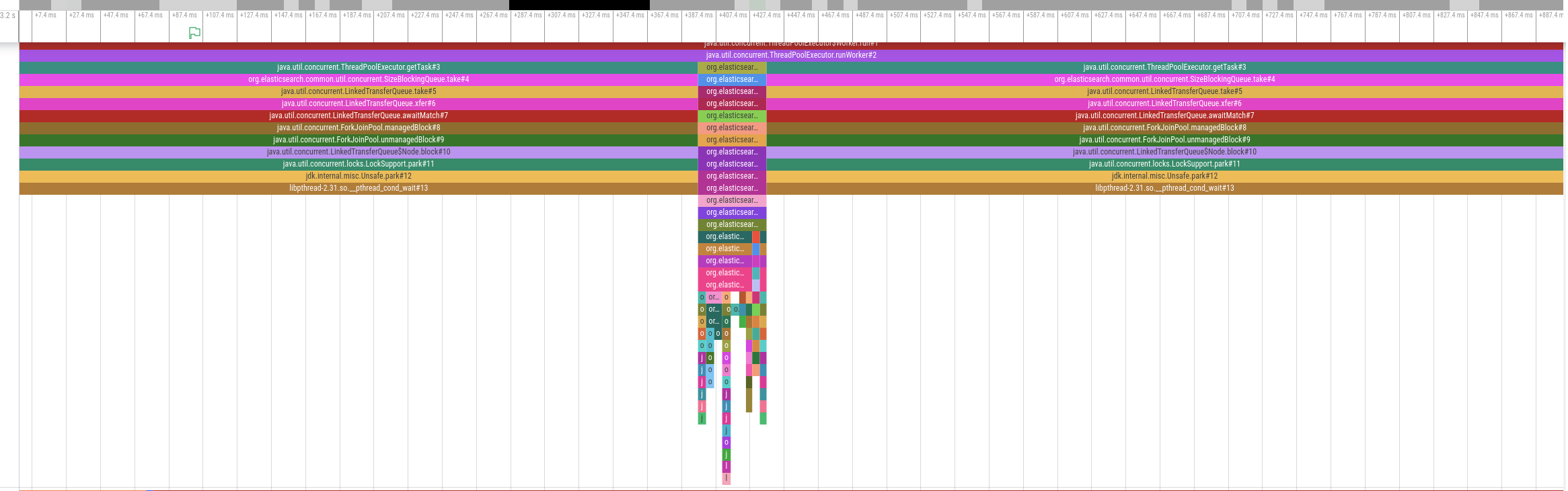
I wrote a program that parses the perf output file and injects the stacktraces into the on-CPU profile to provide a complete picture:
While this looks promising upon first glance, the two profiles are completely misaligned. The on-CPU profile at the beginning indicates that the thread pool is waiting for new tasks (i.e. it’s idle), yet we see several page faults occuring, which can’t be right. Therefore, the two profiles must be misaligned on the time axis. So, how exactly do both profilers get their timestamps?
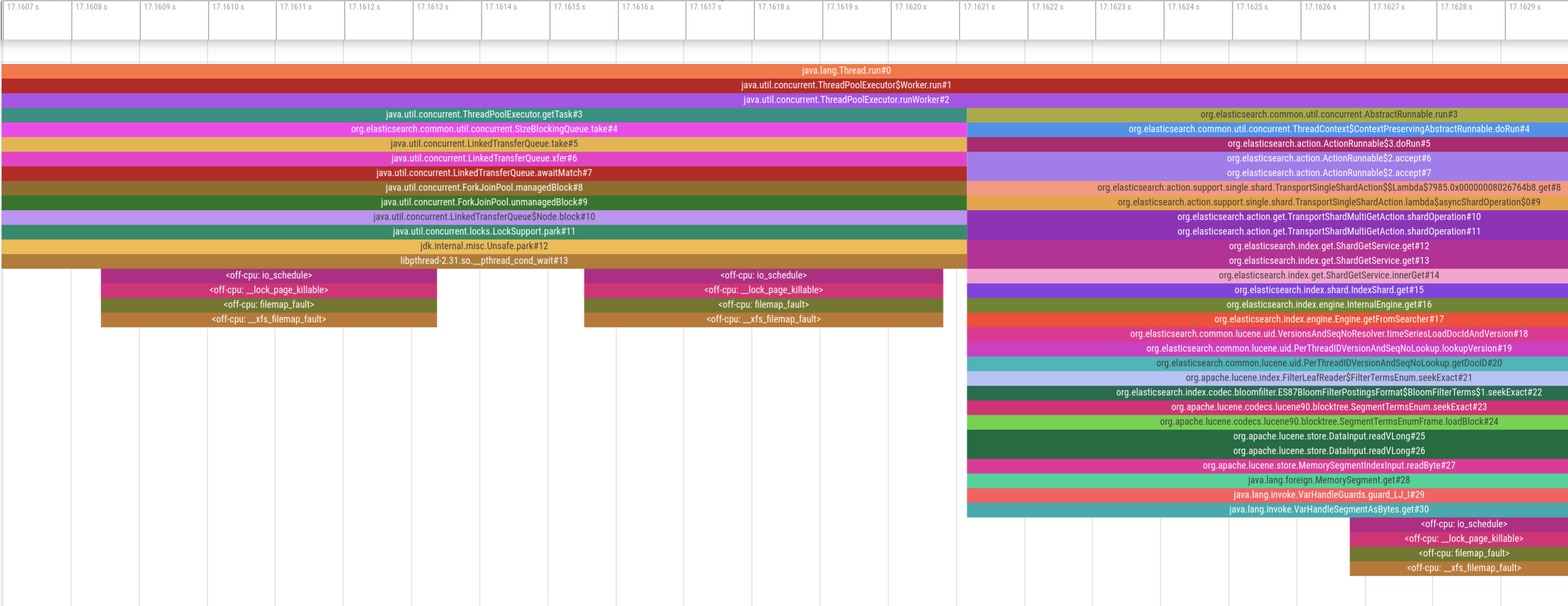
perf record allows to control the clock with the –clock-id parameter. Several clocks are supported, among which we picked CLOCK_MONOTONIC. However, the clock in async profiler is based on the rdtsc instruction on Intel CPUs and non-configurable. rdtsc is basically a hardware counter on the CPU and an interesting topic on its own. For our purposes it’s sufficient to know that the two profilers use different clock sources. Therefore, I’ve raised an issue to add configurable clock sources to async-profiler which Andrei Pangin was kind enough to implement. With async-profiler 2.10 (not yet released as of October 2023) we can use --clock monotonic and force the same clock source in both profilers. This gives us aligned stack traces that combine both on-CPU and off-CPU states:
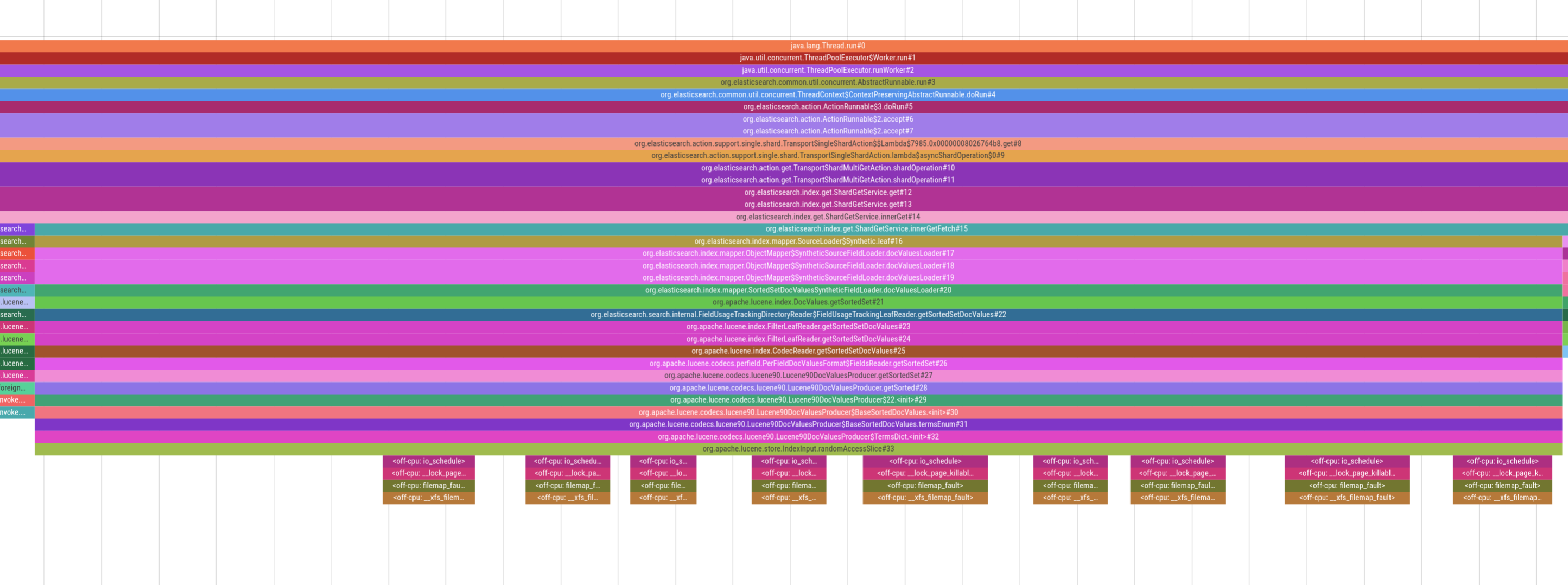
For example, in the picture above we see heavy page-faulting when accessing doc values in Lucene, which is the underlying search engine library that Elasticsearch uses. Being able to visualize this behavior allows us to provide an accurate diagnosis of the situation and then implement appropriate mitigations. Note that some stacktraces might still not be perfectly aligned because perf is tracing whereas async-profiler is sampling. But despite this caveat, seeing on-CPU and off-CPU behavior of an application has still proven extremely valuable when analyzing latency.
Downsampling Profiles
Written on Thu, Jul 20, 2023
I currently work on the backend of Elastic Univeral Profiling, which is a fleet-wide continuous profiler. At Elastic we live the concept of space-time, which means that we regularly get to experiment in a little bit similar vein to Google’s 20% time. Mostly recently, I’ve experimented with possibilities to either store less profiling data or query data in a way that allows us to reduce latency. The data model consists basically of two entities:
- Every time our agent captures a stack trace sample, we store this as a profiling event. Each profiling event contains a timestamp, metadata and a reference to a stacktrace index.
- Stacktraces (and a few related data) are stored in separate indices, which we need to retrieve via key-value lookups.
Experiment
When we create a flamegraph in the UI, we filter for a sample of the relevant events and then amend them with the corresponding stacktraces via key-value lookups. These key-value lookups take a significant amount of the overall time so I’ve randomly downsampled stacktraces, put them in separate indices and benchmarked whether the smaller index size led to a reduction in latency. Unfortunately, I could not observe any improvements.
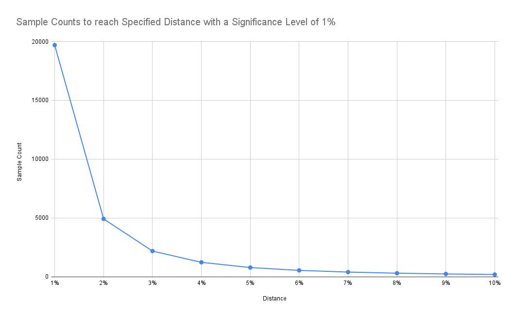
Therefore, I’ve pivoted to better understand the sample size we have chosen to retrieve raw data for flamegraphs (it’s 20.000 samples). The formula to determine the sample size is derived from the paper Sample Size for Estimating Multinomial Proportions. The paper describes an approach to determine the sample count for a multinomial distribution (i.e. stackstraces) with a specified significance level α and a maximum distance d from the true underlying distribution. We have chosen α=0.01 and d=0.01. The formula to calculate sample size n is calculated as:
n=1.96986/d²
The value 1.96986 for the significance level α=0.01 is taken directly from the paper. If you don’t have access, see also this post for more background.
If we are accepting a higher distance from the underlying distribution, we can see that required sample size reduces significantly:
Results
As expected, latency drops as we increase the tolerated distance. Note that the y-axis in the chart below is log-scale:
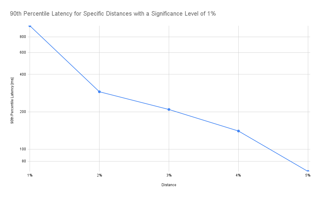
According to the chart above, accepting a 2% distance (instead of 1%) results in a drop of the 90th percentile latency from 982ms to 289ms, i.e. it takes 70% less time to retrieve the data. In addition, the frontend also needs to process only a fraction of the data.
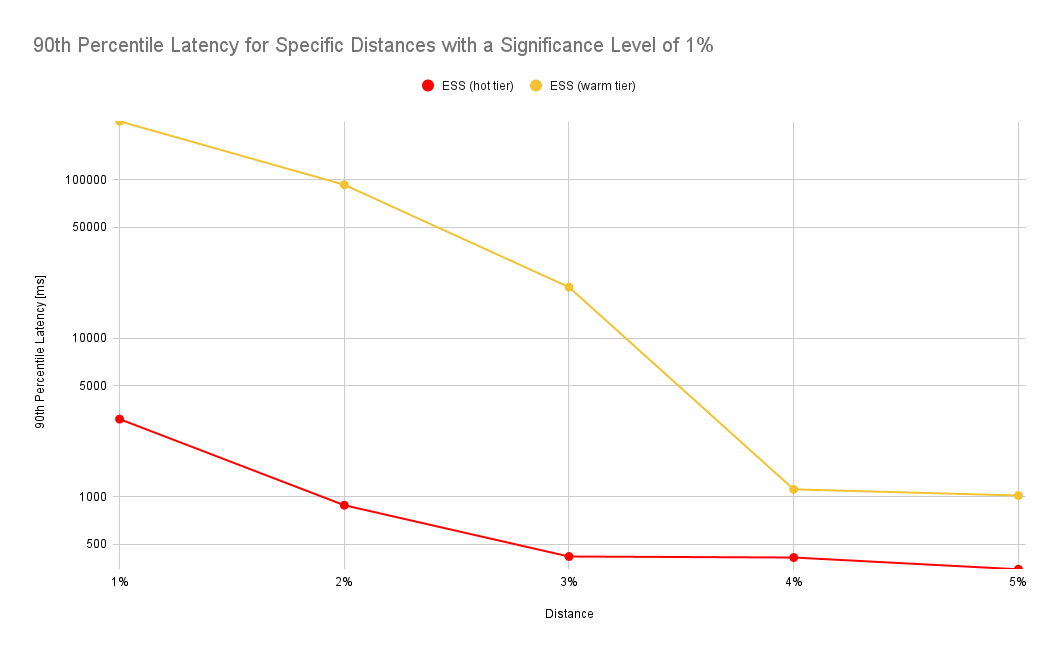
The numbers look similar for a different experiment where we force all indices to be on the hot or warm tier of a cluster. In this benchmark we’ve used a different scenario where we’ve queried a much larger data set covering an entire month whereas in the prior experiment we’ve only queried a day worth of data:
Evaluation
The results look promising but this begs the question whether a 2% distance is acceptable in practice. Therefore, we’ve compared flamegraphs with different distances visually. So let’s look first at our baseline.
20.000 samples (1% distance)
This is the full flamegraph:
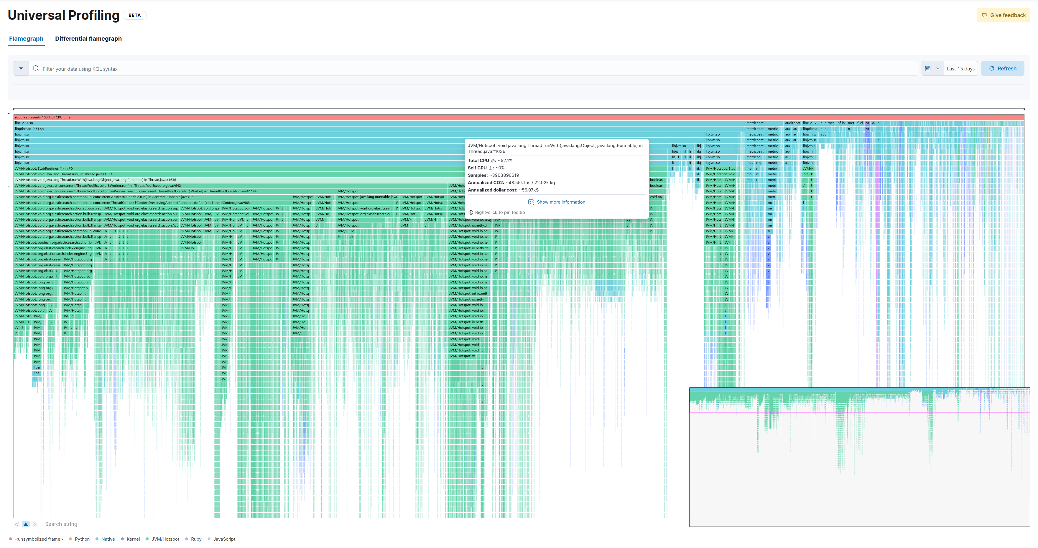
Let’s zoom in a few levels. We’ll select the following method:
And this is how the respective flamegraph looks like:
4.925 samples (2% distance)
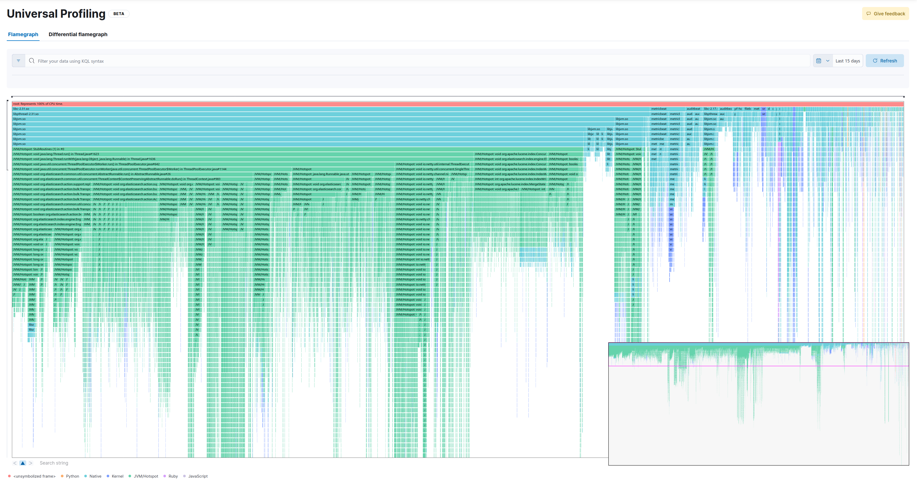
This is the full flamegraph:
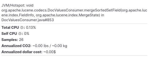
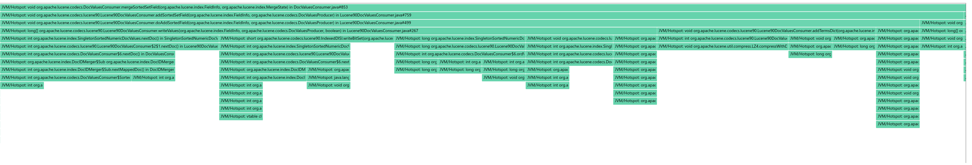
Now let’s drill down into the same method as in the baseline:

As we can see, we lose some samples which take up less CPU (in this example the widest stackframe at the top of the entire zoomed-in screen represents 26 samples). While this would probably not make much difference for most practical applications, there’s also a psychological component to it (Can I trust my profiler?).
The key problem is that stacktraces are not equally distributed but instead skewed heavily:
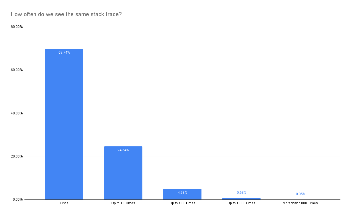
Therefore, it is much more likely that we eliminate one of the stacktraces that make up a spike (show up only once in the most extreme case) despite keeping the statistical properties promised by the sample size estimator. Nevertheless, relaxing constraints might still be a worthwhile option to reduce latency.